7. Deep Learning Basic Course

7.1 Machine Learning Introduction

7.1.1 Overview

Artificial Intelligence (AI) is a new technological science focused on the theories, methods, technologies, and applications used to simulate, extend, and augment human intelligence.

AI encompasses various fields such as machine learning, computer vision, natural language processing, and deep learning. Among them, machine learning is a subfield of AI, and deep learning is a specific type of machine learning.

Since its inception, AI has seen rapid development in both theory and technology, with expanding application areas, gradually evolving into an independent discipline.

7.1.2 What Machine Learning is

Machine Learning is the core of AI and the fundamental approach to enabling machine intelligence. It is an interdisciplinary field involving probability theory, statistics, approximation theory, convex analysis, algorithmic complexity, and more.

Deep learning is a subfield of machine learning that focuses on how computers can acquire new knowledge or skills by simulating or replicating human learning behaviors. It also involves reorganizing existing knowledge structures to continuously improve their own performance. From a practical perspective, machine learning involves training models using data and making predictions with those models.

Take AlphaGo as an example—it was the first AI program to defeat a professional human Go player and later a world champion. AlphaGo operates based on deep learning, which involves learning the underlying patterns and hierarchical representations from sample data to gain insights.

7.1.3 Types of Machine Learning

Machine learning is generally classified into supervised learning and unsupervised learning, with the key distinction being whether the dataset’s categories or patterns are known.

• Supervised Learning

Supervised learning provides a dataset along with correct labels or answers. The algorithm learns to map inputs to outputs based on this labeled data. This is the most common type of machine learning.

For instance, in image recognition, a large number of images of dogs can be labeled as “dog.” The machine learns to recognize dogs in new images through this data.

• Unsupervised Learning

Unsupervised learning involves providing the algorithm with data without labels or known answers. All data is treated equally, and the machine is expected to uncover hidden structures or patterns.

For example, in image classification, if you provide a set of images containing cats and dogs without any labels. The algorithm will analyze the data and automatically group the images into two categories—cat images and dog images—based on similarities.

7.2 Machine Learning Library Introduction

There are many machine learning frameworks available. The most commonly used include PyTorch, TensorFlow, MXNet, and PaddlePaddle.

7.2.1 Pytorch

Torch is an open-source machine learning framework under the BSD License, widely used for its powerful multi-dimensional array operations. PyTorch is a machine learning library based on Torch but offers greater flexibility, supports dynamic computation graphs, and provides a Python interface.

Unlike TensorFlow’s static computation graphs, PyTorch uses dynamic computation graphs, which can be modified in real-time according to the needs of the computation. PyTorch allows developers to accelerate tensor operations using GPUs, build dynamic graphs, and perform automatic differentiation.

7.2.2 TensorFlow

TensorFlow is an open-source machine learning framework designed to simplify the process of building, training, evaluating, and saving neural networks. It enables the implementation of machine learning and deep learning concepts in the simplest way. With its foundation in computational algebra and optimization techniques,

TensorFlow allows for efficient mathematical computations. It can run on a wide range of hardware—from supercomputers to embedded systems—making it highly versatile. TensorFlow supports CPU, GPU, or both simultaneously. Compared to other frameworks, TensorFlow is best suited for industrial deployment, making it highly appropriate for use in production environments.

7.2.3 PaddlePaddle

PaddlePaddle, developed by Baidu, is China’s first open-source, industrial-grade deep learning platform. It integrates a deep learning training and inference framework, a library of foundational models, end-to-end development tools, and a rich suite of supporting components. Built on years of Baidu’s R&D and real-world applications in deep learning, PaddlePaddle is powerful and versatile.

In recent years, deep learning has achieved outstanding performance across many fields such as image recognition, speech recognition, natural language processing, robotics, online advertising, medical diagnostics, and finance.

7.2.4 MXNet

MXNet is another high-performance deep learning framework that supports multiple programming languages, including Python, C++, Scala, and R. It offers data flow graphs similar to those in Theano and TensorFlow and supports multi-GPU configuration. It also includes high-level components for model building, comparable to those in Lasagne and Blocks, and can run on nearly any hardware platform—including mobile devices.

MXNet is designed to maximize efficiency and flexibility. As an accelerated library, it provides powerful tools for developers to take full advantage of GPUs and cloud computing. MXNet supports distributed deployment via a parameter server and can scale almost linearly across multiple CPUs and GPUs.

7.3 YOLO26 Model

7.3.1 Yolo Model Series Introduction and Comparison

• YOLO Series

YOLO (You Only Look Once) is a One-stage, deep learning-based regression approach to object detection.

Before the advent of YOLOv1, the R-CNN family of algorithms dominated the object detection field. Although the R-CNN series achieved high detection accuracy, its Two-stage architecture limited its speed, making it unsuitable for real-time applications.

To address this issue, the YOLO series was developed. The core idea behind YOLO is to redefine object detection as a regression problem. It processes the entire image as input to the network and directly outputs Bounding Box coordinates along with their corresponding class labels. Compared to traditional object detection methods, YOLO offers faster detection speed and higher average precision.

• YOLO26

YOLO26 is the next-generation real-time object detection model introduced by Ultralytics. Built upon the foundation of previous YOLO versions, it features significant optimizations that deliver substantial improvements in both detection speed and accuracy.

Core Features of YOLO26

1. Simplified Architecture: Removes Distribution Focal Loss (DFL) to streamline bounding box regression and enhance export compatibility.

2. End-to-End Inference: Utilizes an NMS-free (Non-Maximum Suppression) design to directly output detection results, significantly reducing latency and deployment complexity.

3. Training Enhancements: Introduces Progressive Loss Balancing (ProgLoss) and Small Target-Aware Label Assignment (STAL) to improve the stability of small object detection.

4. Optimizer Innovations: Utilizes the MuSGD optimizer, which combines the strengths of SGD and Muon to accelerate model convergence.

5. Multi-Task Support: Features a unified framework that supports object detection, instance segmentation, pose estimation, oriented object detection, and image classification.

6. Edge Optimization: Supports FP16/INT8 quantization, enabling low-latency, real-time inference on edge devices such as the NVIDIA Jetson.

7. Performance: Achieves high precision on benchmarks such as COCO, delivering up to a 43% increase in CPU inference speed compared to previous generations.

7.3.2 YOLO26 Model Structure

• Components

1. Convolutional Layer: Feature Extraction

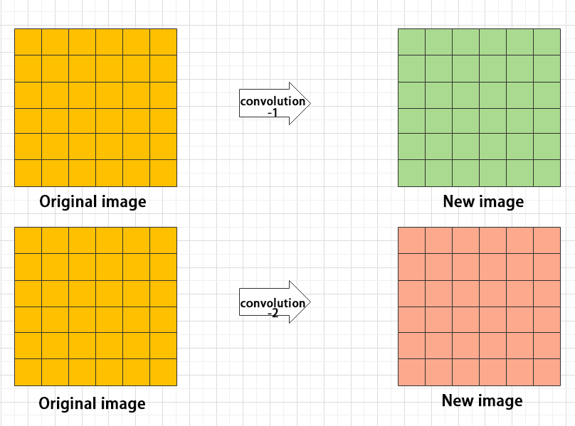
Convolution is the process where an entity at multiple past time points does or is subjected to the same action, influencing its current state. Convolution can be divided into convolution and multiplication.

Convolution can be understood as flipping the data, and multiplication as the accumulation of the influence that past data has on the current data. The data flipping is done to establish relationships between data points, facilitating the calculation of accumulated influence with a proper reference.

In YOLOv8, the data to be processed is images, which are two-dimensional in computer vision. Accordingly, the convolution is two-dimensional convolution. The purpose of 2D convolution is to extract features from images. To perform 2D convolution, it is necessary to understand the convolution kernel.

The convolution kernel is the unit region over which convolution calculation is performed each time. The unit is pixels, and the convolution sums the pixel values within the region. Typically, convolution is done by sliding the kernel across the image, and the kernel size is manually set.

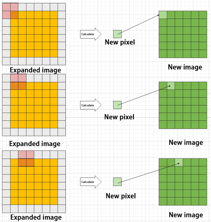
When performing convolution, depending on the desired effect, the image borders may be padded with zeros or extended by a certain number of pixels, then the convolution results are placed back into the corresponding positions in the image.

For example, a 6×6 image is first expanded to 7×7, then convolved with the kernel, and finally the results are filled back into a blank 6×6 image.

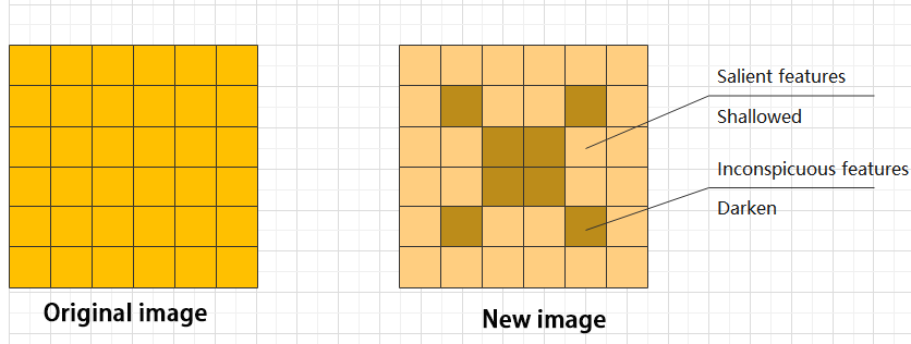
2. Pooling Layer: Feature Amplification

The pooling layer, also called downsampling layer, is usually used together with convolution layers. After convolution, pooling performs further sampling on the extracted features. Pooling includes various types such as global pooling, average pooling, max pooling, etc., each producing different effects.

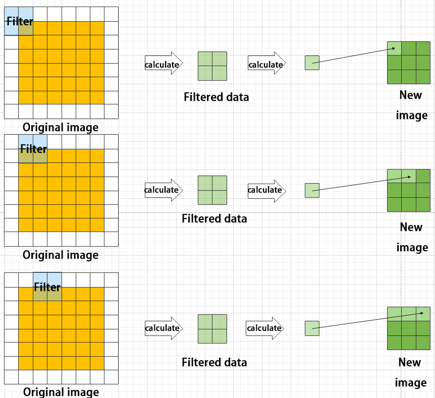
To make it easier to understand, max pooling is used here as an example. Before understanding max pooling, it is important to know about the filter, which is like the convolution kernel—a manually set region that slides over the image and selects pixels within the area.

Max pooling keeps the most prominent features and discards others. For example, starting with a 6×6 image, applying a 2×2 filter for max pooling produces a new image with reduced size.

3. Upsampling Layer: Restoring Image Size

Upsampling can be understood as “reverse pooling.” After pooling, the image size shrinks, and upsampling restores the image to its original size. However, only the size is restored, and the pooled features are also modified accordingly.

For example, starting with a 6×6 image, applying a 3×3 filter for upsampling produces a new image.

4. Batch Normalization Layer: Data Regularization

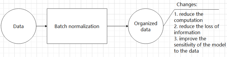
Batch normalization means rearranging the data neatly, which reduces the computational difficulty of the model and helps map data better into the activation functions.

Batch normalization reduces the loss rate of features during each calculation, retaining more features for the next computation. After multiple computations, the model’s sensitivity to the data increases.

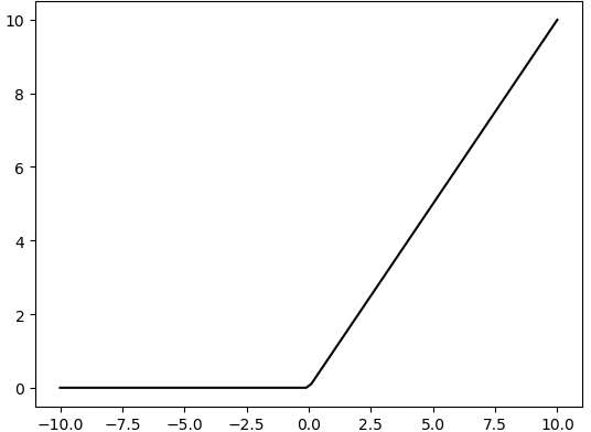
5. ReLU Layer: Activation Function

Activation functions are added during model construction to introduce non-linearity. Without activation functions, each layer is essentially a matrix multiplication. Every layer’s output is a linear function of the previous layer’s input, so no matter how many layers the neural network has, the output is just a linear combination of the input. This prevents the model from adapting to actual situations.

There are many activation functions, commonly ReLU, Tanh, Sigmoid, etc. Here, ReLU is used as an example. ReLU is a piecewise function that replaces all values less than 0 with 0 and keeps positive values unchanged.

6. ADD Layer: Tensor Addition

Features can be significant or insignificant. The ADD layer adds feature tensors together to enhance the significant features.

7. Concat Layer: Tensor Concatenation

The Concat layer concatenates feature tensors to combine features extracted by different methods, thereby preserving more features.

• Composite Elements

When building a model, using only the basic layers mentioned earlier can lead to overly lengthy, disorganized code with unclear hierarchy. To improve modeling efficiency, these basic elements are often grouped into modular units for reuse.

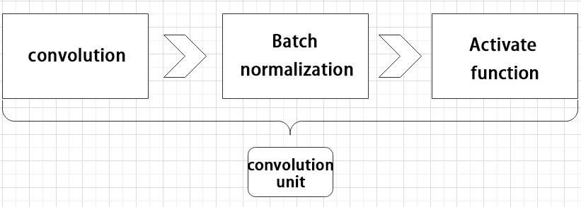
1. Convolutional Block

A convolutional block consists of a convolutional layer, a batch normalization layer, and an activation function. The process follows this order: convolution → batch normalization → activation.

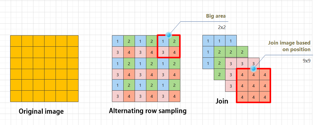
2. Strided Sampling and Concatenation Unit（Focus）

The input image is first divided into multiple large regions. Then, small image patches located at the same relative position within each large region are concatenated together to form a new image. This effectively splits the input image into several smaller images. Finally, an initial sampling is performed on the images using a convolutional block.

As shown in the figure below, for a 6×6 image, if each large region is defined as 2×2, the image can be divided into 9 large regions, and each contains 4 small patches.

By taking the small patches at position 1 from each large region and concatenating them, a 3×3 image can be formed. The patches at other positions are concatenated in the same way. Ultimately, the original 6×6 image is decomposed into four 3×3 images.

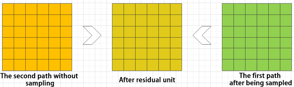
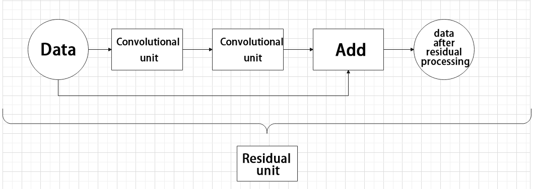
3. Residual Block

The residual block enables the model to learn subtle variations in the image. Its structure is relatively simple and involves merging data from two paths.

In the first path, two convolutional blocks are used to extract features from the image. In the second path, the original image is passed through directly without convolution. Finally, the outputs from both paths are added together to enhance learning.

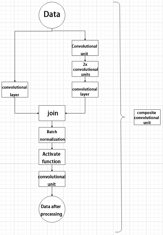
4. Composite Convolutional Block

In YOLO26, a key feature of the composite convolutional block is its customizable design, allowing convolutional blocks to be configured as needed. This structure also uses two paths whose outputs are merged.

The first path contains a single convolutional layer for feature extraction, while the second path includes 2𝑥+1 convolutional blocks followed by an additional convolutional layer. After sampling and concatenation, batch normalization is applied to standardize the data, followed by an activation function. Finally, a convolutional block is used to process the combined features.

5. Composite Residual Convolutional Block

The composite residual convolutional block modifies the composite convolutional block by replacing the 2𝑥 convolutional blocks with 𝑥 residual blocks. In YOLO26, this block is also customizable, allowing residual blocks to be tailored according to specific requirements.

6. Composite Pooling Block

The output from a convolutional block is simultaneously passed through three separate max pooling layers, while an additional unprocessed copy is preserved. The resulting four feature maps are then concatenated and passed through a convolutional block. By processing data with the composite pooling block, the original features can be significantly enhanced and emphasized.

7.3.3 YOLO26 Workflow

This section explains the model’s processing flow using the concepts of prior boxes, predicted boxes, and anchor boxes.

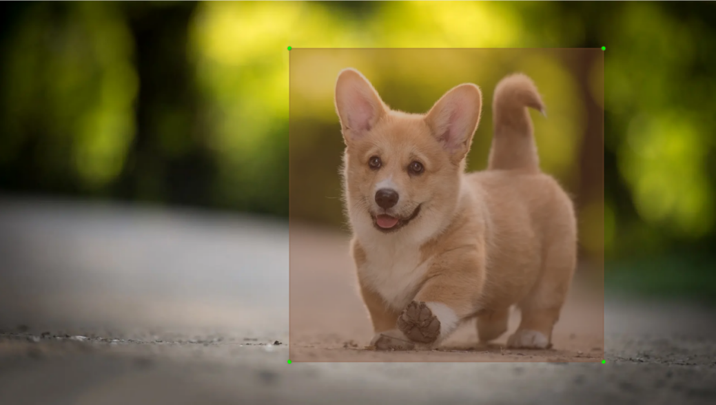
• Prior Box

When an image is fed into the model, predefined regions of interest must be specified. These regions are marked using prior boxes, which serve as initial bounding box templates indicating potential object locations in the image.

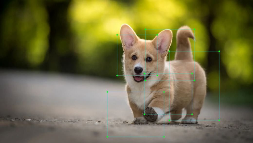
• Predicted Box

Predicted boxes are generated by the model as output and do not require manual input. When the first batch of training data is fed into the model, the predicted boxes are automatically created. The center points of predicted boxes tend to be located in areas where similar objects frequently appear.

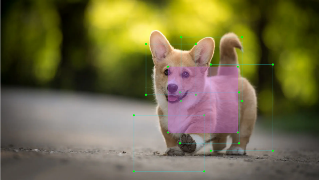
• Anchor Box

Since predicted boxes may have deviations in size and location, anchor boxes are introduced to correct these predictions.

Anchor boxes are positioned based on the predicted boxes. By influencing the generation of subsequent predicted boxes, anchor boxes are placed around their relative centers to guide future predictions.

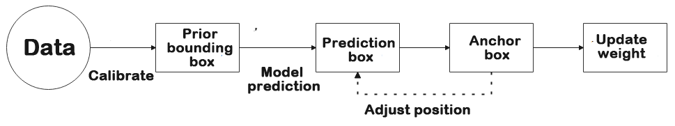
• Project Process

Once the bounding box annotations are complete, prior boxes appear on the image. When the image data is input into the model, predicted boxes are generated based on the locations of the prior boxes. Subsequently, anchor boxes are generated to adjust the predicted results. The weights from this round of training are then updated in the model.

With each new training iteration, the predicted boxes are influenced by the anchor boxes from the previous round. This process is repeated until the predicted boxes gradually align with the prior boxes in both size and location.

7.4 YOLO26 Model Training

7.4.1 Image Collection and Labeling

Training a YOLO model requires a substantial dataset. Therefore, data collection and annotation must be performed first to prepare for subsequent model training.

• Image Collection

1. Power on the robot and establish a connection via VNC remote desktop software.

2. Click the desktop icon to open a terminal.

~/.stop_ros.sh

3. Enter the command to launch the depth camera service.

 ros2 launch peripherals depth_camera.launch.py

4. Open a new terminal window and execute the following command to create a directory for storing the dataset.

mkdir -p ~/my_data

5. Execute the command to launch the image collection utility.

cd ~/software/collect_picture && python3 main.py

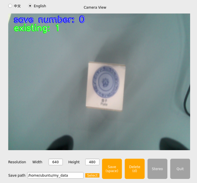
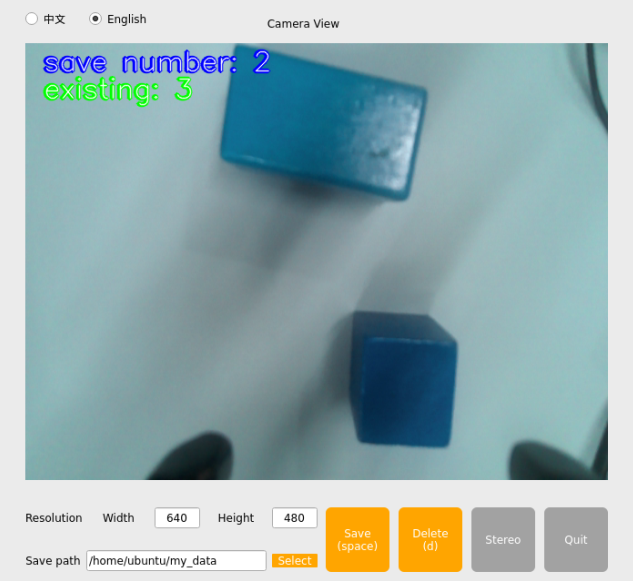
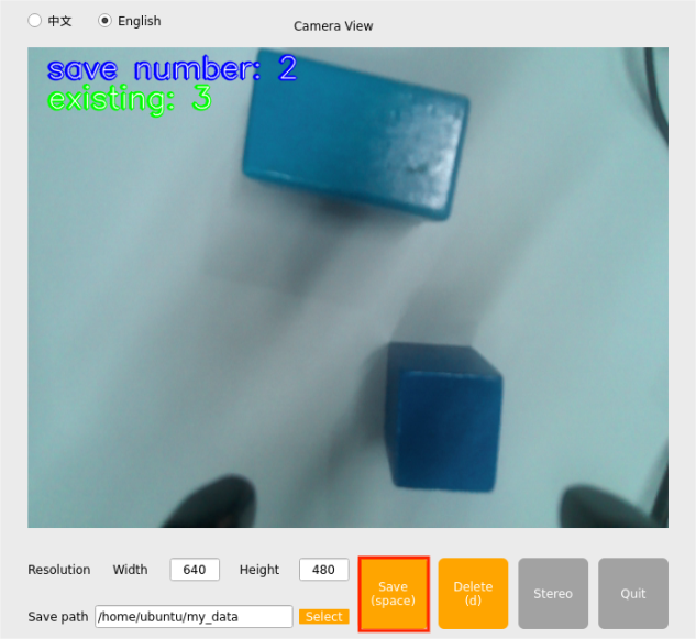
The save number displayed in the upper-left corner indicates the current image ID or the index of the saved image. The existing represents the total number of images saved so far.

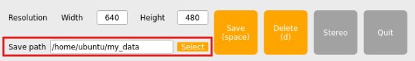
6. Click Select and modify the destination path to the newly created directory.

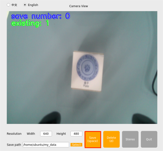
7. Once the target directory is selected, click Choose.

8. Place the target object within the field of view of the camera. Click the Save (space) button or press the Spacebar to capture and save the current frame.

9. After clicking Save (space) or pressing the Spacebar, a JPEGImages folder will automatically be generated inside the /home/ubuntu/my_data directory to store the captured images.

Note

To enhance model robustness, capture the target object from various distances, rotational angles, and tilt angles.

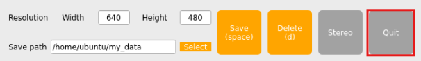
10. Once image collection is complete, click the Quit button to close the utility.

11. Open a terminal and run the command to verify the saved images.

cd ~/my_data/JPEGImages && ls

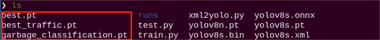
12. Press the key combination Ctrl + C in all open terminal windows to terminate the processes. This completes the image collection workflow.

• Image Labeling

Image annotation is a critical step following data collection. Annotating the dataset defines ground truth boundaries and object classes, enabling the model to learn prominent features and generalize effectively to new, unseen images.

Note

Terminal commands are strictly case-sensitive. The Tab key can be used for keyword auto-completion.

1. Open a terminal and execute the command to launch the annotation software.

python3 ~/software/roLabelImg/roLabelImg.py

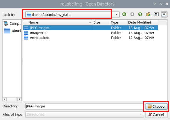
2. In the software interface, click File in the top-left corner, select Open Dir, navigate to the image repository directory, and click Choose.

3. Click File in the top-left corner and select Change default saved Annotation dir to update the destination path to the Annotations directory inside the my_data folder.

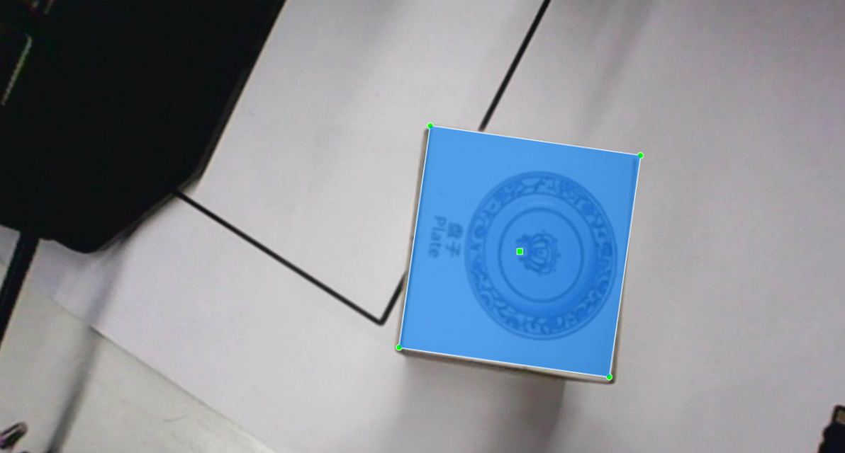
4. Click View in the top-left corner and select Advanced Mode to enable the oriented bounding box function for rotated annotations.

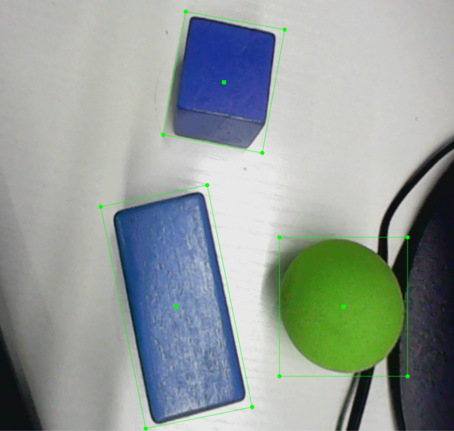
5. Use the following shortcuts for efficient labeling. Press E to create a rotated bounding box, D for the next image, and A for the previous image. For adjustments, use C for a minor clockwise rotation, X for a minor counterclockwise rotation, V for a major clockwise rotation, and Z for a major counterclockwise rotation. Click the Save icon on the left panel after completing each image.

Note

The C and X keys must be used to rotate and precisely align the bounding box with the contours of the object. Improper alignment will degrade downstream detection accuracy.

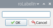
6. Assign a class name to the target object in the dialog box. After entering the class name, click OK to save the label.

7. Press the D key to proceed to the next image. Once all images are labeled, click the close icon in the top-right corner of the window to exit the software.

7.4.2 Data Format Conversion

• Preparation

Before proceeding with this section, image collection and annotation must be completed. For detailed instructions, refer to 7.4.1 Image Collection and Labeling.

Before feeding the dataset into the YOLO26 model for training, defining the object classes and converting the annotation files into the required format is mandatory.

• Format Conversion

Before starting this section, image collection and annotation must be completed.

Note

Terminal commands are strictly case-sensitive. The Tab key can be used for keyword auto-completion.

1. Open a new terminal and run the command to view the configuration file. If the file does not exist, it can be created directly using this command.

 gedit ~/my_data/classes.names

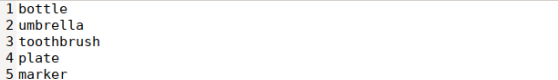
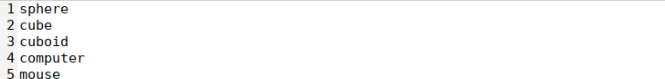
2. Write the designated class name, left, into the text file. If dealing with multiple distinct classes, enter each class name on a separate line.

Note

The class name added here must exactly match the label defined in the “roLabelImg” annotation software.

3. After editing, press Ctrl + S to save the changes and close the editor.

4. Return to the terminal window, execute the format conversion command, and press Enter.

python3 ~/third_party_ros2/yolo/xml2yolo_obb.py --data ~/my_data --yaml ~/my_data/data.yaml

5. The parameters utilized in the command are defined below.

(1) my_data: Represents the custom annotated dataset folder. The specified directory path must match the actual location.

(2) data.yaml: Defines the data structural configuration for the dataset conversion. As indicated by the command, the output file will be saved inside the my_data directory.

7.4.3 Model Training

Note

Terminal commands are strictly case-sensitive. The Tab key can be used for keyword auto-completion.

• Preparation

Following the format conversion, the next phase is model training. Ensure that the formatted dataset is fully prepared by referencing section 7.4.2 Data Format Conversion.

• Model Training

1. Start the robot and connect it to the VNC remote control software.

2. Click the desktop icon on the system desktop to open a command line terminal.

3. Run the following command to navigate to the designated workspace directory.

cd ~/third_party_ros2/yolo/yolo26

5. Execute the training command to begin the optimization process.

python3 train.py --img 640 --batch 64 --epochs 300 --data ~/my_data/data.yaml --weights yolo26n.pt

Within the training arguments:

–img specifies the input resolution.

–batch defines the batch size per iteration.

–epochs determines the total training cycles.

–data points to the dataset configuration path.

–weights designates the initial pre-trained weights file.

These configuration parameters can be modified based on specific project requirements. Increasing the number of epochs generally enhances model accuracy and reliability, though it extends total computation time.

Once model training concludes, the output directory path will be displayed in the terminal. The weights and evaluation results for this session are saved in the /home/ubuntu/runs/detect/train3 directory.

Note

The exact generation path varies depending on prior runs. The latest output folder can be located within the “runs/detect/train” directory.

7.4.4 Object Detection

A custom deployment model is obtained after extensive training cycles. To review the comprehensive workflow, refer to sections 7.4.1 Image Collection and Labeling through 7.4.3 Model Training.

• Operation Steps

1. Click the desktop icon to open a terminal window, then run the command to stop the default background application service.

~/.stop_ros.sh

2. Execute the following command to copy the newly trained best.pt file to the ~/third_party_ros2/yolo directory. The target source folder name may vary based on the training iteration and should be adjusted accordingly.

cp ~/runs/detect/train3/weights/best.pt ~/third_party_ros2/yolo

3. Open the launch file using the text editor command.

gedit ~/ros2_ws/src/example/example/yolo_detect/yolo_detect_demo.launch.py

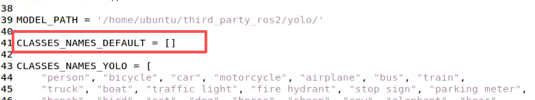
Locate the CLASSES_NAMES_DEFAULT parameter and insert the trained class name, left, enclosed in double quotation marks. Save the file and close the editor.

4. Launch the object detection node using the provided command.

ros2 launch example yolo_detect_demo.launch.py model_name:=best

• Detection Results

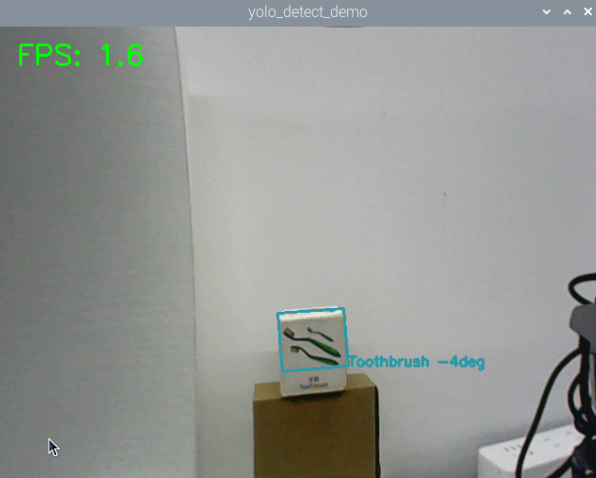
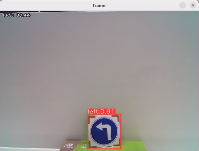
Place a target road sign within the camera field of view. When successfully detected, a bounding box will frame the target on the video stream, accompanied by its class label and the inference confidence score.

7.5 Waste Classification Card Model

Product names and reference directory paths mentioned throughout this documentation are subject to change depending on the actual hardware version and configuration.

Training on the embedded robot controller board is discouraged when handling larger datasets due to RAM constraints and I/O hardware limitations. Utilizing a desktop or laptop equipped with a dedicated graphics card is highly recommended. The core training workflow remains identical, requiring only the deployment of the corresponding software environment.

This section serves as a direct reference guide for training custom deep learning models.

7.5.1 Preparation

1. Prepare a workstation or laptop computer. Ensure a wireless network card and standard peripherals are available if a desktop computer is utilized.

2. Install and launch the VNC remote desktop client based on the procedures detailed in previous chapters.

7.5.2 Model Deployment

1. Execute the command to terminate the app service.

~/.stop_ros.sh

2. Launch the trash classification object detection pipeline.

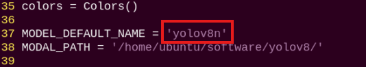
ros2 launch example yolo_detect_demo.launch.py model_name:=best_garbage_26

• Detection Results

Place a waste classification card within the camera’s field of view. Upon recognition, a bounding box will highlight the object in the preview window, displaying the identified class name and its associated detection confidence score.