6. OpenCV Computer Vision Course
6.1 Application Course
6.1.1 Testing and Usage of USB Camera
The camera needs to be used in various vision-based gameplay, allowing for quick deployment to meet these requirements.
Connect Device
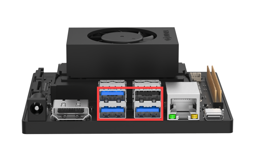
Connect the USB camera to any of ports highlighted in the below red box on Jetson Orin Nano.
Start Testing
Note
The input command should be case sensitive, and the “Tab” key can be used to complement the key words.
If you’re using the pre-installed system image, you can located the corresponding program by referring the content in “2. Configuration Guide -> Flashing System Using an SSD -> 5. System Image Directory Instructions”.
Power on Jetson Orin Nano board, then connect to the remote system desktop via NoMachine.
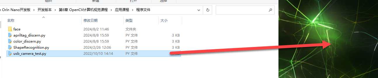
Drag the program file “usb_camera_test.py” in “Program Files” into the system desktop.
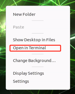
Right click on a blank area of the system desktop to select “Open in Terminal” to open the terminal:
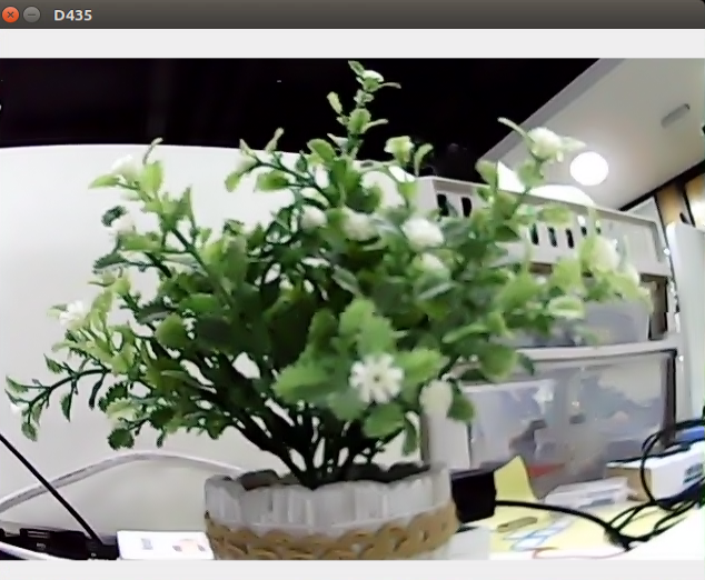
Enter the command and press Enter to run the program.
python3 usb_camera_test.py

If you need to close the program, press the shortcut key “Ctrl+C” in the terminal to exit the program.
Code Analysis
The image below shows the screenshot of the example test code:
import cv2
if __name__ == "__main__":
cap = cv2.VideoCapture(0)
if cap.isOpened():
window_handle = cv2.namedWindow("D435", cv2.WINDOW_AUTOSIZE)
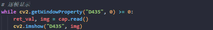
# 逐帧显示
while cv2.getWindowProperty("D435", 0) >= 0:
ret_val, img = cap.read()
cv2.imshow("D435", img)
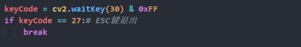
keyCode = cv2.waitKey(30) & 0xFF
if keyCode == 27:# ESC键退出
break
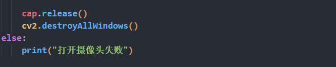
cap.release()
cv2.destroyAllWindows()
else:
print("打开摄像头失败")
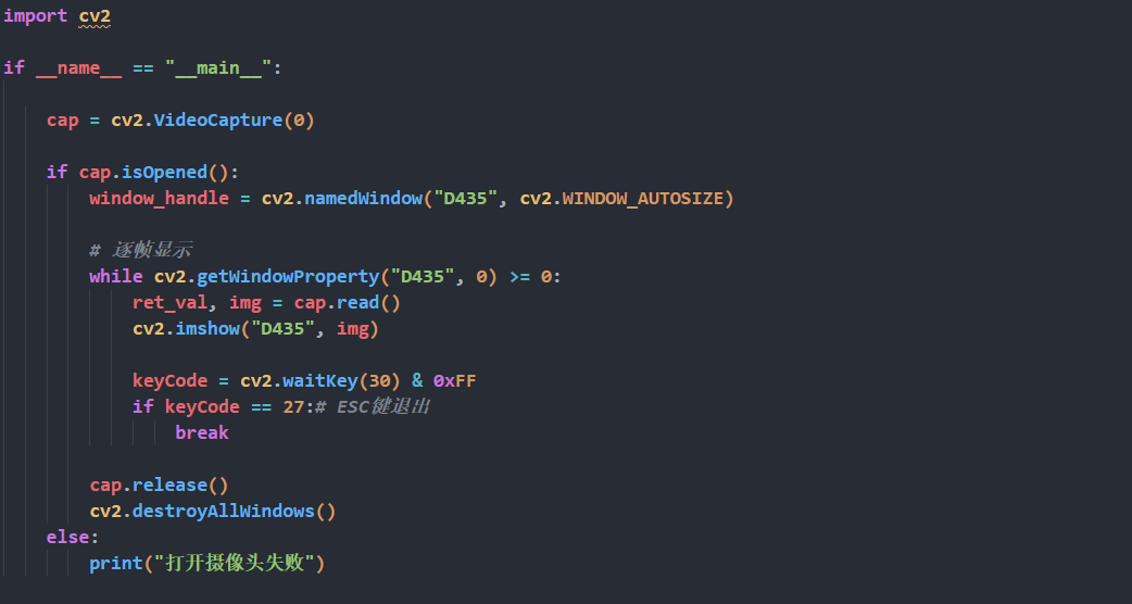
Import opencv library:
import cv2

Select the camera to be used. Since we only have one camera connected, you only need to set the parameter to 0.
cap = cv2.VideoCapture(0)

Set up the window for display the live camera feed, with the window name “D435” and video size as “cv2.WINDOW_AUTOSIZE”
if cap.isOpened():
        window_handle = cv2.namedWindow("D435", cv2.WINDOW_AUTOSIZE)

Read the transmitted camera image data and display it.
# 逐帧显示
        while cv2.getWindowProperty("D435", 0) >= 0:
            ret_val, img = cap.read()
            cv2.imshow("D435", img)
Set up to close the window by pressing the “Esc” key.
keyCode = cv2.waitKey(30) & 0xFF
            if keyCode == 27:# ESC键退出
                break
If the camera is not detected or if another error occurs, “Failed to open camera” will be printed.
cap.release()
        cv2.destroyAllWindows()
    else:
        print("打开摄像头失败")
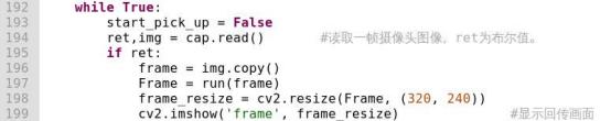
6.1.2 Color Recognition
Program Logic
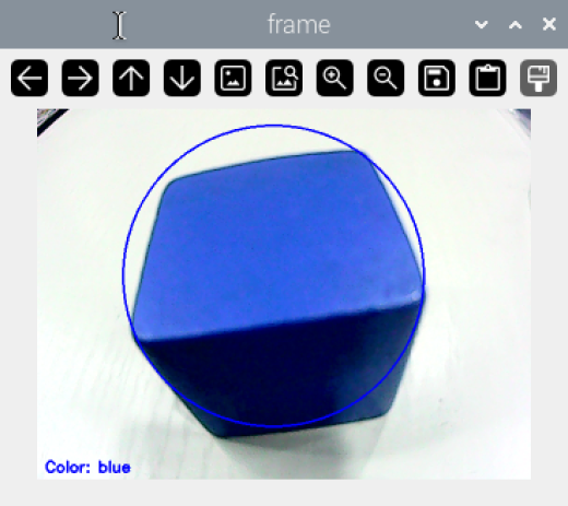
The color recognition function allows the camera to identify objects based on red, green, and blue colors. When the target color is detected, the object is outlined with a circle of the corresponding color in the transmitted image.
The color is processed through the Lab color space. First, the RGB color space is converted to Lab, followed by binarization. After applying operations like dilation and erosion, the contour containing only the target color is obtained. This contour is then enclosed with a circle, enabling the recognition of the object’s color.
Operation Steps
Note
If you use the system image we provide, you can find the corresponding program in the folder “3. Basic Operation Course -> 3.2 Introduction to System Desktop .”
This method requires that the purchased kit includes the expansion board.
Prior to operations, you need to transfer the routine “color_discern.py” stored in “6. OpenCV Computer Vision Course\ Program Files” to the Jetson Orin Nano.
For the file transfer method, you can refer to the content in “3. Basic Operation Course”.
Note
The input command should be case sensitive, and the “Tab” key is able to implement the key works.
Open Nocmahine. Double click on  , or use the shortcut key to open the terminal. After entering the command, it will start color recognition.
python3 color_discern.py

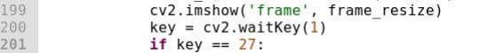
At this point, the live camera feed will display in the terminal. When recognizing the objects of red, green or blue, the target object will be outlined with a circle of the corresponding color. To close this program, press “Esc”.
Program Analysis
The program is stored in:
/home/ubuntu/Opencv/color_discern.py
1. Import Library File
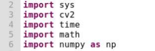
Import the cv2, sys, time math libraries from openCV, and also import and instantiate the numpy library as np.
2. Set Color Threshold
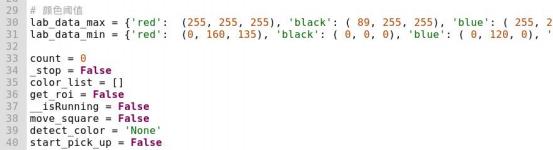
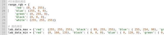
Set the threshold for color recognition. In the routine, the target threshold for the target recognition color by the camera has been set (the default color model in OpenCV is BGR, i.e, 'red': (0, 0, 255),'blue': (255, 0, 0),'green': (0, 255, 0) ), and then a range is set for the threshold, as shown in the figure below:
3. Acquiring the Recognition Frame
The second parameter calls the
VideoCapture()function to define the camera object, where the parameter 0 represents the first camera. If there are multiple cameras, the parameter can be changed to 1, 2, 3, etc.

In the while loop, use the
read()function of the camera object to capture a frame of the video and display it.
Then wait for 1 unit of time. If the “ESC” key is detected during this period, exit and close the window.
Call the
destroyAllWindows()function to close all image windows.

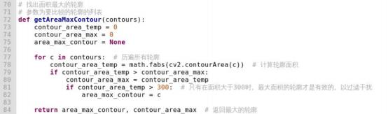
4. Color Recognition
After capturing the recognition frame through the camera, use the getAreaMaxContour() function to process the frame and obtain the object’s contour. The specific processing method is shown in the image below:
Then, use the putText() function from the cv2 library to print the recognition information, as shown in the image below (partial function screenshot):

The parameter analysis for the code cv2.putTextimg, "Color: " + detect_color, (10, img.shape[0] - 10), cv2.FONT_HERSHEY_SIMPLEX, 0.65, draw_color, 2 is as follows:
First parameter image: Represents the target image.
Second parameter Color: " + detect_color: Specifies the text string to be drawn.
Third parameter 10, img.shape[0] - 10: The coordinates for the bottom-left corner of the text string in the image.
Fourth parameter cv2.FONT_HERSHEY_SIMPLEX: Specifies the font type for printing.
Fifth parameter 0.65: Represents the font size.
Sixth parameter draw_color: Represents the font color.
Seventh parameter 2: Specifies the thickness of the font.
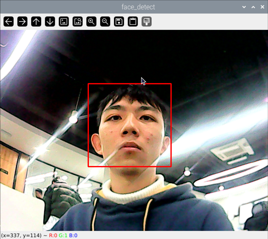
6.1.3 Face Detection
Program Logic
Firstly, load the pre-trained Haar feature classifier model. Then create a window and capture the video stream. Process each frame by converting it to a grayscale image and applying the Haar feature classifier for face detection. The detected face locations will be marked with rectangular boxes on the original image. The processed image will be displayed in real-time it the window.
Operation Steps
If you use the system image we provide, you can find the corresponding program in the folder “3. Basic Operation Course -> 3.2 Introduction to System Desktop .”
This method requires that the purchased kit includes the expansion board.
Prior to operations, you need to transfer the routine “face.p andhaarcascade_frontalface_default.xml” stored in “6. OpenCV Computer Vision Course\ Program Files” to the Jetson Orin Nano.
For the file transfer method, you can refer to the content in “3. Basic Operation Course”.
Note
The input command should be case sensitive, and the “Tab” key is able to implement the key works.
Open Nocmahine. Double click on
 , or use the shortcut key to open the terminal. After entering the command, it will start face detection.
python3 face.py

At this point, the terminal will display the live camera feed, and the camera will automatically outline the detected face, as shown in the image below. To close this program, press the “ESC” key.
Program Analysis
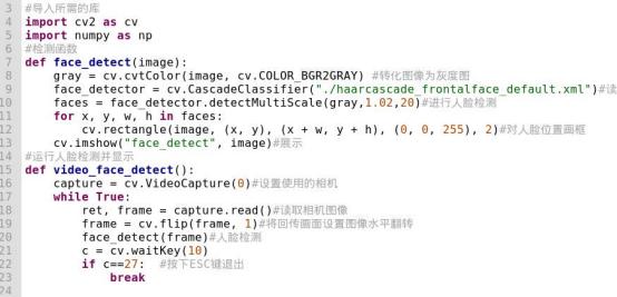
The program is stored in:
/home/ubuntu/Opencv/face/face.py
#导入所需的库
import cv2 as cv
import numpy as np
#检测函数
def face_detect(image):
gray = cv.cvtColor(image, cv.COLOR_BGR2GRAY) #转化图像为灰度图
face_detector = cv.CascadeClassifier("./haarcascade_frontalface_default.xml")#读取人脸数据
faces = face_detector.detectMultiScale(gray,1.02,20)#进行人脸检测
for x, y, w, h in faces:
cv.rectangle(image, (x, y), (x + w, y + h), (0, 0, 255), 2)#对人脸位置画框
cv.imshow("face_detect", image)#展示
#运行人脸检测并显示
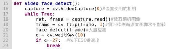
def video_face_detect():
capture = cv.VideoCapture(0)#设置使用的相机
while True:
ret, frame = capture.read()#读取相机图像
frame = cv.flip(frame, 1)#将回传画面设置图像水平翻转
face_detect(frame)#人脸检测
c = cv.waitKey(10)
if c==27: #按下ESC键退出
break
Import Library File
Import the cv2 library from openCV, and import and instantiate the numpy library as np.
import cv2 as cv
import numpy as np

Main Function Analysis
1. Real-time Face Detection
if __name__ == '__main__':
    video_face_detect()#实时检测人脸

Invoke the
video_face_detect()function to run the face detection and display it.
def video_face_detect():
    capture = cv.VideoCapture(0)#设置使用的相机
    while True:
        ret, frame = capture.read()#读取相机图像
        frame = cv.flip(frame, 1)#将回传画面设置图像水平翻转
        face_detect(frame)#人脸检测
        c = cv.waitKey(10)
        if c==27:  #按下ESC键退出
            break
In the
video_face_detect()function, use theVideoCapture()function from the cv2 library to define the camera object.
capture = cv.VideoCapture(0)

The parameter 0 in VideoCapture() represents the first camera. If there are multiple cameras, you can use parameters 1, 2, 3, etc.
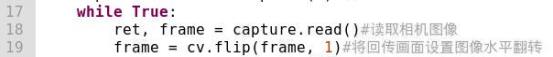
In the while loop, use the
read()function of the camera object to capture a frame of the video, and then use theflip()function from the cv2 library to horizontally flip the transmitted camera.
while True:
        ret, frame = capture.read()#读取相机图像
        frame = cv.flip(frame, 1)#将回传画面设置图像水平翻转
        face_detect(frame)#人脸检测
Call the
face_detect()function to perform detection on the image.
face_detect(frame)
def face_detect(image):
    gray = cv.cvtColor(image, cv.COLOR_BGR2GRAY) #转化图像为灰度图
    face_detector = cv.CascadeClassifier("./haarcascade_frontalface_default.xml")#读取人脸数据
    faces = face_detector.detectMultiScale(gray,1.02,20)#进行人脸检测


In the image detection function, to speed up detection, first use the
cvtColor()function from the cv2 library to convert the source image to grayscale. In this function, the first parameter image is the source image, and cv.COLOR_BGR2GRAY is the color conversion code. Next, use theCascadeClassifier()function to load the face detection data. Call thedetectMultiScale()function to detect faces. In this function:
The first parameter gray is the image to be detected.
The second parameter 1.02 is the scaling factor for the detection window, which enlarges by 2% in each successive scan.
The third parameter 20 is the minimum number of adjacent rectangles required to form a detection.

Finally, use the
rectangle()function to draw boxes around the detected faces, and use theimshow()function to display the annotated image in the feedback window.Then, wait for 10 units of time. If the “ESC” key is detected during this period, exit and close the window.

2. Exiting Face Detection
Call the destroyAllWindows() function to close all the image windows.

6.1.4 Tag Recognition
Program Logic
When the tag card is recognized by the camera, the corresponding ID of the tag will be displayed in the transmitted image after processing.
AprilTag is similar to barcodes and QR codes. As a visual position marker, it can be use for quickly detecting tags and calculating their relative positions, meeting real-time requirements. The principle of tag recognition is as follows:
Step 1: Image Acquisition and Processing:
First, initialize the camera. After capturing the image, process it by copying, remapping, and displaying it. Convert the BGR format image to grayscale.
Step 2: Tag Detection:
Next, obtain the coordinates of the four corners of the tag and draw the contours of the AprilTag.
Step 3: Tag Information Retrieval:
Then, within the identified quadrilateral, determine the pixel coordinates to further verify the reliability of the encoding. Match the tag with a known encoding library. After filtering and validation, calculate the tag’s ID and rotation angle.
Step 4: Highlight Detected Tags and Activate the Buzzer:
Finally, convert the coordinates of the detected tags to their pre-scaled coordinates, and determine if it is the largest tag. Highlight the recognized tag and activate the buzzer.
Operation Steps
If you use the system image we provide, you can find the corresponding program in the folder “3. Basic Operation Course -> 2. Introduction to System Desktop .”
This method requires that the purchased kit includes the expansion board.
Prior to operations, you need to transfer the routine “apriltag_discern.py” stored in “6. OpenCV Computer Vision Course\ Program Files” to the Jetson Orin Nano.
For the file transfer method, you can refer to the content in “3. Basic Operation Course”.
Note
The input command should be case sensitive, and the “Tab” key is able to implement the key works.
Open Nocmahine. Double click on
 , or use the shortcut key to open the terminal. Enter the command to install the “apriltag” package.
pip3 install apriltag -i <https://pypi.tuna.tsinghua.edu.cn/simple>
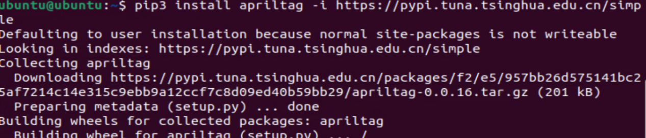
Install gtk-module:
sudo apt-get install libcanberra-gtk-module

Enter the command to start tag recognition.
python3 apriltag_discern.py

At this point, the terminal’s live camera feed will open, and the camera will recognize tags within its visual range. When a tag is detected, it will be highlighted on the feedback screen, and its ID information will be printed in the lower-left corner, as shown in the image below:
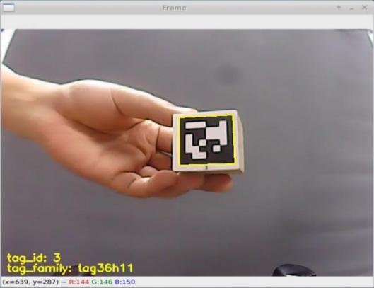
To close the program, press “Esc”.
Program Analysis
The program is stored in:
/home/ubuntu/Opencv/apriltag_discern.py
1. Import Library File
Import the cv2 and apriltag libraries from openCV, and import and instantiate the numpy library as np.
2. Tag Recognition

AprilTag recognition primarily uses the cv2 library functions drawContours() and putText(). Here’s a breakdown of how drawContours() is used:
The drawContours() function is used to draw the contours of the tag. The parameters are as follows:
The first parameter img is the image on which the contours are to be drawn.
The second parameter [np.array(corners, np.int)] is the contours themselves. In Python, this is a list containing an array of the contour points.
The third parameter -1 specifies which contours to draw. -1 indicates that all contours in the list should be drawn.
The fourth parameter (0, 255, 255) is the color of the contours, specified in BGR (Blue, Green, Red) format. Here, (0, 255, 255) represents yellow.
The fifth parameter 2 is the thickness of the contour lines. 2 indicates a line width of 2 pixels. Using -1 instead would fill the contours with the specified color.

The putText() function is used to display text on an image. For example:
The first parameter img is the input image on which the text will be displayed.
The second parameter "tag_id:" + str(tag_id) is the text to be added.
The third parameter (10, img.shape\[0\] - 30) The coordinates of the bottom-left corner of the text.
The fourth parameter cv2.FONT_HERSHEY_SIMPLEX is the font type used for the text.
The fifth parameter 0.65 is the size of the font.
The sixth parameter [0, 255, 255] is the color of the text, in BGR (Blue, Green, Red) format. Here, it represents yellow.
The seventh parameter 2 is the thickness of the font.
6.1.5 Shape Recognition
Program Logic
Recognize the object of different shapes by the camera. When the shape of an object is identified (triangle, rectangle, circle), the object with the corresponding shape will be outlined in the transmitted image.
First, the color of the recognized object is identified. Then, the object’s corner points are detected. The obtained corner points are analyzed and distinguished according to the number of corners corresponding to different shapes, as shown in the table below:
| Shape | Number of corners |
|---|---|
| 0 | Circle |
| 3 | Triangle |
| 4 | Rectangle |
Then, the identified shape is outlined using the corresponding shape in the image.
Operation Steps
If you use the system image we provide, you can find the corresponding program in the folder “3. Basic Operation Course -> 2. Introduction to System Desktop .”
This method requires that the purchased kit includes the expansion board.
Prior to operations, you need to transfer the routine “ShapeRecognize.py” stored in “6. OpenCV Computer Vision Course\ Program Files” to the Jetson Orin Nano.
For the file transfer method, you can refer to the content in “3. Basic Operation Course”.
Note
The input command should be case sensitive, and the “Tab” key is able to implement the key works.
Open Nocmahine. Double click on
 , or use the shortcut key to open the terminal. Enter the command to start shape recognition.
python3 ShapeRecognition.py

At this point, the terminal’s live camera feed will display. When a green object is recognized, the corresponding object will be outlined with a red line, and the name of the object’s shape will be displayed above, as shown in the image below:
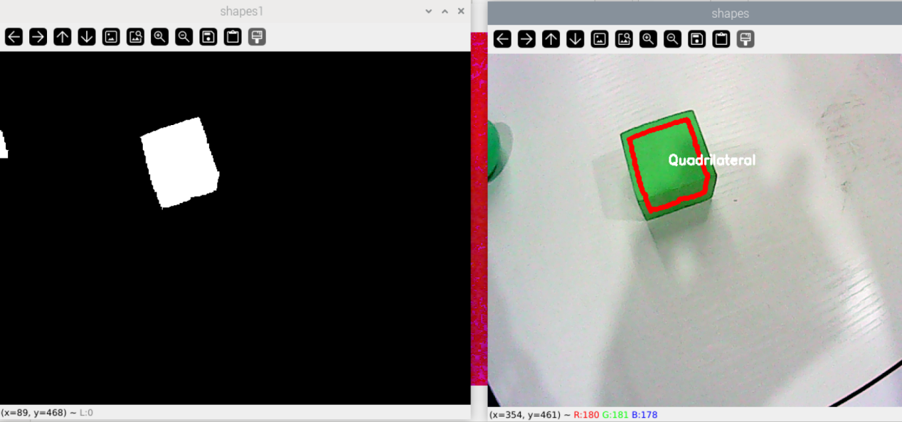
To close this program, press “q”.
Program Analysis
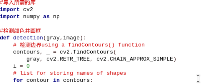
The program is stored in:
/home/ubuntu/Opencv/ShapeRecognition.py
#导入所需的库
import cv2
import numpy as np
#检测颜色并画框
def detection(gray,image):
    # 检测边界using a findContours() function
    contours, _ = cv2.findContours(
        gray, cv2.RETR_TREE, cv2.CHAIN_APPROX_SIMPLE)
    i = 0
    # list for storing names of shapes
    for contour in contours:
1. Import Library File
Import the cv2 library from openCV, and import and instantiate the numpy library as np.
import cv2
import numpy as np
2. Detect Object Color and Draw Frame
Define a function to detect the color of the object and outline its contour. The specific code is shown in the image below:
#检测颜色并画框
def detection(gray,image):
    # 检测边界using a findContours() function
    contours, _ = cv2.findContours(
        gray, cv2.RETR_TREE, cv2.CHAIN_APPROX_SIMPLE)
    i = 0
    # list for storing names of shapes
    for contour in contours:
        # here we are ignoring first counter because
        # findcontour function detects whole image as shape
        #if i == 0:
            #i = 1
           # continue
        # 计算边长数量cv2.approxPloyDP() function to approximate the shape
        approx = cv2.approxPolyDP(
            contour, 0.06 * cv2.arcLength(contour, True), True)
        # 根据检测到边缘画边using drawContours() function
        cv2.drawContours(image, [contour], 0, (0, 0, 255), 5)
    try:
        # 寻找中心点finding center point of shape
        M = cv2.moments(contour)
        if M['m00'] != 0.0:
            x = int(M['m10'] / M['m00'])
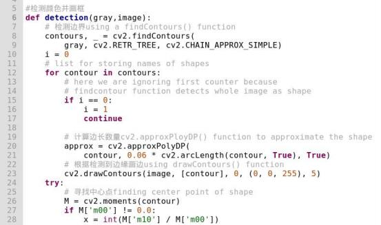
Call the findContours() function from the cv2 library to detect the boundaries of the object and assign the value 0 to i, as shown in the image below:
def detection(gray,image):
    # 检测边界using a findContours() function
    contours, _ = cv2.findContours(
        gray, cv2.RETR_TREE, cv2.CHAIN_APPROX_SIMPLE)
    i = 0
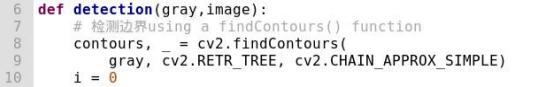
At the same time, set up a loop to iterate through the detection data.
Then, use the approxPolyDP() function from the cv2 library to calculate the number of sides of the object.
approx = cv2.approxPolyDP(
            contour, 0.06 * cv2.arcLength(contour, True), True)

Then, use the drawContours() function to draw the edge lines.
cv2.drawContours(image, [contour], 0, (0, 0, 255), 5)

The parameters of the drawContours() function are as follows:
The first parameter, image, represents the target image.
The second parameter, [contours], represents the input contour set, where each contour is composed of a vector of points.
The third parameter, 0, specifies which contour to draw. If this parameter is negative, all contours will be drawn.
The fourth parameter, (0, 0, 255), specifies the color of the contour.
The fifth parameter, 5, denotes the line width of the contour. If it is negative or set to CV_FILLED, the contour will be filled.
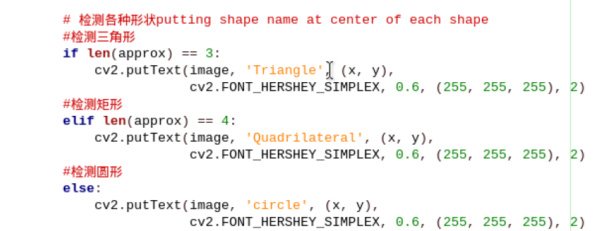
3. Shape Classification
Determine the shape based on the number of identified sides. If the number of sides is 3, it is a triangle, and the feedback screen will display Triangle. If the number of sides is 4, it is a rectangle, and the feedback screen will display Quadrilateral. Otherwise, it is a circle, and the feedback screen will display Circle.
6.2 Basic Course
6.2.1 Computer Vision and OpenCV Introduction
How robots “see” the world
For artificial intelligence, the ability to see is essential. And how robots see the world involves machine vision, an important branch of artificial intelligence.
Machine vision is the idea that the robot takes human’s place to measure and make judgments. The captured target will be converted into image signal by image sensor, CMOS or CCD, and then the image signal will be transferred to the specialized image processing system which will convert the image signal into digitized signal according to the pixel distribution, brightness, color, etc.
Image system perform various operations on these signals to extract the features of the target, so as to control the device in the field based on the judgments.
Machine vision technology is commonly applied in intelligent transport system and intelligent housing system.
Image Recognition Introduction
Image recognition is a crucial technique that uses computer to process and analyze the image so as to recognize different targets.
Similar to human eyes, machine image recognition starts at the point where there is huge variance or sudden change, and the features will recognized one by one. Our brain controls our eyes to collect the major features of the image and filter the redundant information, and then integrate the major features into the complete visual image.
The process of computer image recognition is no different from that of human image recognition, which is divided into four steps.
Acquire information: the light signal, sound signal, etc., are converted into electric signal by the sensors to acquire the information
Image preprocessing: perform smoothing, denoising, etc., on the image to highlight the major features of the image.
Feature extracting and selecting: extract and select the image features, which is the pivotal step.
Image classification: make the recognition rules that is design classifier based on the training result to get the main category of the features so as to improve the recognition accuracy.
Image recognition is mostly applied in remote sensing image recognition
and robot vision.
OpenCV Introduction
OpenCV (Open Source Capture Vision) is a computer vision library for free handling various tasks about image and video, for example display the image collected by the camera and make the robot recognize the real object.
OpenCV is more eminent than PIL, the built-in image processing library in Python. OpenCV provides complete Python interfaces, and Python3.5 and opencv-python library file have been integrated in the provided image system.
How Images are Stored in Computer
How the images are stored in computer after they are recognized?
In general, a picture is composed of pixels and each pixel can be represented by R, G and B components within 0-255. OpenCV stores each pixel as a ternary array making it convenient to record all information of the image. In addition, OpenCV records the data of three color channels of RGB image in the order of BGR.
Besides, images of other standards (HSV) are stored as multivariate array. An OpenCV image is a two-dimensional or three-dimensional array. An 8-bit grayscale image (black-and-white images) is a two-dimensional array, and a 24-bit BGR image is a three-dimensional array.
For a BGR image, the first value of the element image[0,0,0] represents Y–axis coordinate or the row number(0 represents the top). The second value represents X-axis coordinate or column number (0 represents leftmost ). And the third value represents the color channel.
Same as Python array, these array recording images can be accessed individually to obtain the data of some color channel or capture a region of the image.
6.2.2 Build OpenCV Environment
Install Numpy
Each picture involves several pixels, which results in that a large number of arrays need to be processed in the program. Numpy is a extension library for Python, which handles multi-dimensional arrays more efficiently than Python’s native array structures. Besides, it can improve the readability of codes.
Open command line terminal and then input command “pip install numpy” to install Numpy. For more information about Numpy, please move to the folder “4. Basic Programming Course->4.13 Python Numpy Basic Operation”.
pip install numpy
Install OpenCV
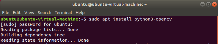
OpenCV package can be obtained from Ubuntu repository. Then refresh the packages index and install the OpenCV package by typing the following commands.
sudo apt update: refresh the packages index
sudo apt update
sudo apt install python3-opencv: Install the package. During installation, input “y” to continue the execution and the complete installation may take 10s.
sudo apt install python3-opencv
Verify the Installation of OpenCV
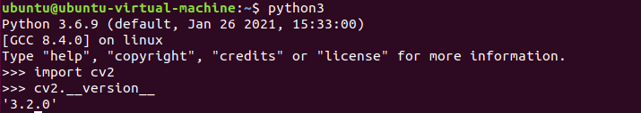
We can import cv2 module to print the version of OpenCV so as to verify whether the installation is successful or not.
python3: enter Pythonimport cv2: import cv2 modulecv2.__version__: check the version
If the version of OpenCV is printed, the installation is successful.
6.2.3 OpenCV Modules and Components
OpenCV Component
OpenCV is composed of several layers of modules.
The bottom layer is the hardware optimization based on HAL (Hardware Acceleration Layer)
Above the bottom layer are the codes contributed by other developers contained in opencv_contrib module. These codes, core of OpenCV, involves most of the high-level functionality.
The next layer are language bindings and sample applications.
The top layer is the interaction between OpenCV and operating system.
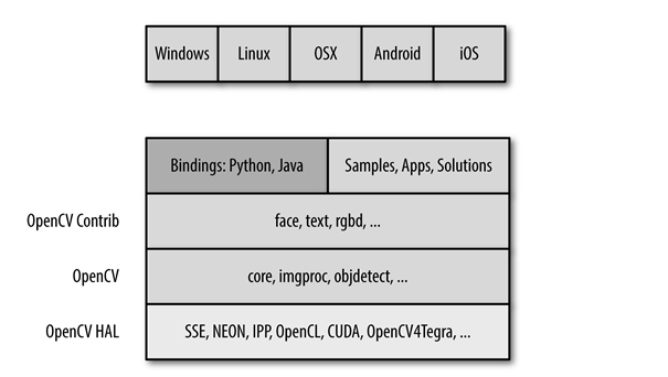
Specific Module of OpenCV
Core: Contain the basic structure and operation of OpenCV library.Improc: Image processing module can transform the basic image, including filtering and convolution.Highgui: Seen as lightweight Windows UI Toolkit, it is divided into imcodecs, videoio and highgui in OpenCV 3.0. It contains user-interaction function used to display the images or simple input.Video: Contain the functions for reading and writing the video streams.Calib3d: Contain the algorithm of the calibration of single, binocular and multiple cameras.Feature2d: Used for the algorithm of feature point detection, description and matching.Objdectect: Contain the algorithm of specific target detection, including human face or passengers. And it can be used to train the detector to detect other objects.Ml: Machine learning module is a comprehensive module that involves a mass of machine learning algorithms which can interact with OpenCV data type.Flann: Flann stands for Fast Library for Approximate Nearest Neighbors, which will be called by the functions in other modules for fast nearest neighbor search in large datasets.GPU: It is segmented into several cuda* modules in OpenCV. GPU module can optimize the functions on CUDA GPU and involves the functions only applicable to GPU. Without GPU, the computing resources cannot be promoted causing that some functions cannot return good results.Photo: A new module that contains the functions of computational photography.Stitching: Also a new module that stitches sophisticated imagesNonfree: It is moved to opencv_contrib/xfeatures2d in OpenCV 3.0. There are some algorithms that is protected by patent and limited in usage in OpenCV, such as SIFT. These algorithms are isolated into their own modules, therefore you need to take special measures to use them in commercial products.Contrib: It involves something new that haven’t been integrated into OpenCV.Legacy: It has been removed from OpenCV 3.0. This module contains some old stuffs that haven’t been completely removed.Ocl: Khronos OpenCL standard. It has been removed from OpenCV 3.0 and replaced by T-API. Similar to GPU module, it realizes Khronos OpenCL standard for open parallel programming.
Compared with GPU module, it has fewer functions, but it aims at providing the parallel devices that can run on any GPU or is powered by Khronos. However, GPU module can only run on Nvidia GPU devices for the reason that it utilizes Nvidia CUDA toolkit to develop.
6.2.4 Picture & Video Loading and Display
Image Reading and Writing
Read image: cv2.imread(Location,Model)
Location——read the location of the image which can be the absolute path and relative path. However pay attention to the usage of the slash in different operating system.
Model——model of image loading. The first model is
cv2.IMREAD_COLORused to load a color picture but will not load Alpha channel(record degree of transparency). The second one is cv2.IMREAD_GRAYSCALE which is used to load a grayscale picture. The third type is cv2.IMREAD_UNCHANGED for loading image and Alpha channel simultaneously.Display image: cv2.imshow(“Name”, Pic)
Name——Display the box name of the image
Pic——Pictures to be displayed(The image read by cv2.imread() has already used before) For example, create a new py file and put the picture named “camera.png” into the same folder. Then input the following codes. After the codes run, the image will be displayed and you can press any key to hide the image.
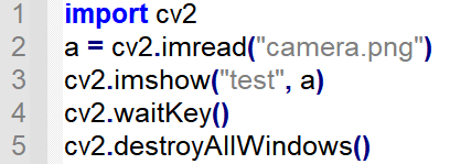
Note
cv2 waitkey() allows users to display a window for given milliseconds or until any key is pressed. And cv2.destroyALLWindows() function will close all the windows.
Video Reading and Writing
Video can be seen as pictures that are switched swiftly. Therefore, video reading is the extension of the image reading and writing. Camera initialization: cv2.VideoCapture(Number)
Number——Serial number of camera, 0 usually.
Read the frame of camera:cap.read()
cap——the camera that has been defined before
Release the resources of the camera: cap.release()
For example, the camera screen will be displayed on the desktop. When q key is pressed, the camera screen will be hidden.
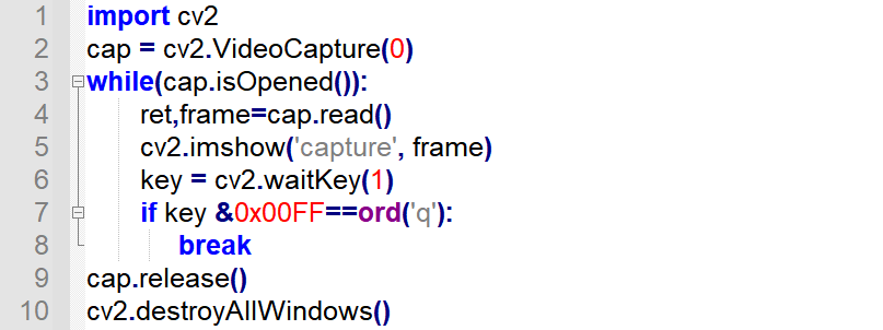
Note
cv2.waitKey(delay) will wait for the input from the keyboard and can be used to refresh the image in the video. “delay” in the bracket indicates the waiting time. When a frame of picture is displayed, the program will display the next frame in “delay” ms.
6.2.5 Image Drawing
Drawing function in OpenCV can be used to draw line, rectangle, circle, etc., and add texts to the designated position of the picture.
Draw Line
Function format: cv2.line(image,pt1,pt2,color,thickness)
Image: Image where the line will be drawnpt1: starting coordinate of the line. The coordinate is represented by a tuples consisting of two values i.e. (X,Y)pt2: ending coordinate of the line. The coordinate is represented by a tuples consisting of two values i.e. (X,Y).Color: The color of the line. And BGR is represented by a tuple. For example, (255, 0, 0) stands for blue.Thickness: The thickness of the line

Draw Rectangle
Function format: cv2.rectangle(image,pt1,pt2,color,thickness)
image: The picture where the rectangle will be drawnpt1: vertex coordinate of the rectangle, (x,y), which is represented by a tuple consisting of two numbers.pt2: The diagonal vertex coordinates of pt1 and its format is similar to that of pt1.color: The color of the rectangle. And BGR is represented by a tuple. For example, (255, 0, 0) stands for blue.thickness: Line thickness. The greater the value, the thicker the line. If the value is negative or cv2.FILLED, a filled rectangle will be drawn.

Draw Circle
Function format: cv2.circle(image,center,radius,color,thickness)
image: The picture where the circle will be drawncenter: The center of the circle, (x,y), which is represented by a tuple consisting of two numbers.radius: The radius of the circle.color: The color of the circle. BGR is represented by a tuple. For example, (255, 0, 0) stands for blue.thickness: Line thickness. The greater the value, the thicker the line. If the value is negative or cv2.FILLED, a filled circle will be drawn.

Draw Polygon
Function format: cv2.polylines(image,pts,isClosed,color,thickness)
image: The picture where the polygon will be drawnpts: The vertex coordinate of the polygon. When several quadrangles are required in a picture, the shape of ndarray is (N,4,2).isClosed: Whether the polygon is closed or not, True generally.color: The color of the polygon. BGR is represented by a tuple. For example, (255, 0, 0) stands for blue.thickness: Line thickness. The greater the value, the thicker the line.

Add Text
Function format: cv2.putText(image,text,pt,font,fontScale,color)
image: The image where the text is added.text: The text contentpt: The coordinate of the upper left corner of the textfont: Font of the textfontScale: Font sizecolor: The color of the text. BGR is represented by a tuple. For example, (255, 0, 0) stands for blue.

6.2.6 Image Basic Operation
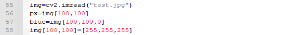
Acquire and Modify the Pixel of the Image
The value of the pixel can be acquired through the coordinate of row and column. For BGR image, an array consisting of blue, green and red values will be returned. For grayscale image, the corresponding intensity will be returned. And the pixel can be modified in this way.
img[x,y]: Acquire the value of some pixel and return its BGR value.img[x,y,index]: Acquire the value of a color channel. The order of the color channel is BGR.img[x,y]=[B,G,R]: Modify the color channel value of this pixel.
Acquire the Image Property
shape: If it is a color picture, acquire the shape of the image and return an array containing the number of row, column and channel. If it is binary image or grayscale image, only the number of row and column will be returned. Through judging whether the returned value contains the number of channel, we can know that it is a grayscale picture or color picture.size: Return the pixel number of the image. The format is “row x column x channel”. The number of channel of the grayscale picture is 1.dtype: Return the data type of the picture

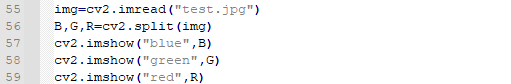
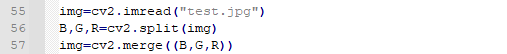
Splitting and Merging of Image Channel
1. Splitting of Image Channel
split: Input the image to be split and return the picture with three individual color channels.
2. Merging of Image Channel
merge: Merge three individual channels, including B, G and R into BGR image with three channel.
Color Space Conversion
There more than 150 ways to convert colors in OpenCV. And BGR is commonly converted into GRAY and HSV. The function format is ·cvtColor(img,flag).**
img: The image converted the color spaceflag: The converted type. For example, cv2.COLOR_BGR2HSV indicates that convert BGR into HSV.

6.2.7 Image Processing—Color Space Conversion
Color Space Introduction
Each frame of the picture is arranged by the pixels that are composed of three color components, including B, G and R.
Color model is also called color space which is a mathematical model using an array to describe color.
Besides the familiar RGB picture, there are other color spaces, including GRAY, Lab, XYZ, YCrCb, HSV, HLS, CIEL*a*b*, CIEL*u*v*, Bayer, etc.
Expertise of each color space is different. Therefore, color space conversion can improve the efficiency of tackling a specific problem.
Color space conversion refers to transform the image from one color space to another color space. For example, convert the picture from RGB to Lab. When extracting the feature of the picture, and calculating the distance, we usually covert the picture from RGB into gray color space. In some applications, it is necessary to convert the color space image into binary image.
Some common color spaces are listed below.
Common Color Space
1. RGB Color Space
The properties of RGB color space are as follow.
1.An RGB color space is an additive color space and the colors are obtained from linear combination of R(red), G(Green) and B(Blue).
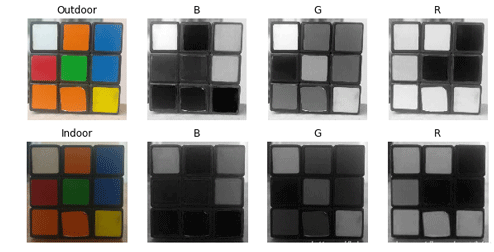
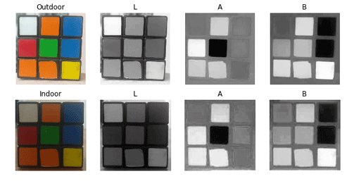
2.The illumination will affect the value of each color channel and these three color channels are related. For better understanding of color space, we can divide the image into R, G and B three components
From the blue channel picture in indoor, blue is similar to white. However, from the blue channel picture in outdoor, there is distinction between blue and white. And this nonuniformity makes color-based segmentation infeasible in color space. In addition, the value of these two pictures are also different. Therefore, there are flaws in RGB color space, including uneven color value and mixed chroma and luminance.
2. Lab Color Space
Similar to RGB, Lab also has three image channels.
L:Luminance channel
a:Color channel a representing colors from green to carmine.
b:Color channel b representing colors from blue to yellow.
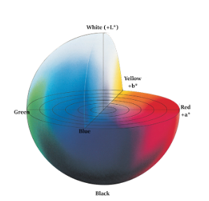
Lab is totally different from RGB color space. In RGB, colors are divided into three channels and each channel contains luminance. While in Lab, colors are divided into L channel only containing luminance, a channel and b channel.
L component: represent the luminance of the pixel. The larger L value, the greater the luminance.
a component: represent the range from red to green.
b component: represent the range from yellow to blue.
In OpenCV, R, G and B value in RGB color space all range from 0 to 255. In Lab color space, L ranges from 0 to 100. When L is 0, the color is black and when it is 100, the color is white. a and b values range from -128 to 127. When both a and b are 0, the color is gray.
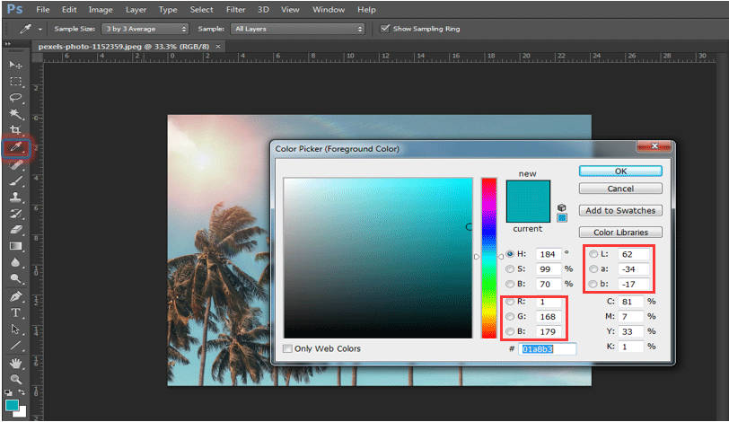
To better assist in your understanding of the comparison between RGB and Lab, operate on PS.
Use eyedropper tool to get the color.
Click the color picker at bottom left corner, the correspondence between Lab and RGB is listed below.
Lab color space has these features:
A perceptually uniform color space align with the way human perceive color.
Independent from device(capture or display)
Widely applied in Adobe Photoshop
It is related to the RGB color space through complex transformation equations
In OpenCV, the image converted into Lab color space is as follow.
3. Ycrcb Color Space
HVS (Human Visual System) is less sensitive to color than to luminance. In traditional RGB color space, three primary colors, RGB, bear the same importance, but luminance is overlooked.
In YCrCb color space, Y represents luminance, and Cr and Cb stand for chroma. Cr indicates red component and Cb indicates blue component. Luminance can reflect how bright or dark a color is, which can be calculated through a weighted sum of the light intensity. The green component has the greatest impact on RGB light while the blue component the least.
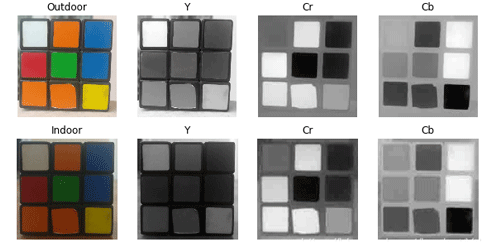
Observations focusing on intensity and color components can be made for LAB for illumination changes. Compared with LAB, the perception difference between red and orange in outdoor is smaller, while white between three components are distinguished.
4. HSV Color Space
HSV color space is vision perception oriented color model which is composed of these three components.
H (hue), S (saturation) and V (value)
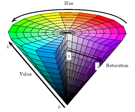
Hue: it is related to the dominant wavelength of light in the mixed spectrum, for example “red orange yellow green blue purple” represents different hues respectively. In the perspective of wavelength, light of different wavelength appear as different colors, i.e. different hues.
Saturation: describes the purity of a color or pertains to the amount of white light mixed with a hue. Pure spectrum is fully saturated, and dark red (red mixed with white) and light purple (purple mixed with white) is not saturated enough. Saturation is inversely proportional to the amount of white light mixed.
Brightness: it reflect the brightness perceived by human and it is relative to the reflection of the object. For a hue, the greater the amount of white mixed in a hue, the greater the value. And the greater the amount of black mixed in a hue, the weaker the brightness.
The most distinguished feature of HSV is that it only employs single channel to describe hue, which make it intuitive to designate a hue. But HSV colors rely on device.
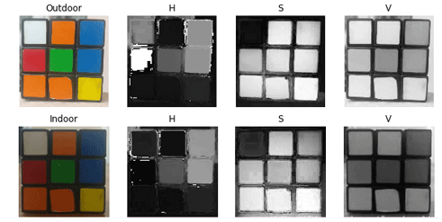
H components in outdoor and indoor are similar, which indicates the color is complete even though the lighting changes.
S components in outdoor and indoor are also similar. V stands for brightness so that it will change as the lighting changes.
The difference of red value between indoor and outdoor is large for the reason that H component represent red by angle ranging from [300,360] and [0,60].
5. Gray Color Space
GRAY color space generally refers to grayscale image, monochromatic image, in which each pixel is processed into 256 gray level from black to white.
These 256 gray levels are represented by the number within [0,255]. “0” indicates pure black, and “255” represents white. Number from 0 to 255 denote dark gray or light gray of different brightness (shade of hue).
Color Conversion
The function below is used to transform color.
dst = cv2.cvtColor( src, code [, dstCn] )
dst represents the output image whose data type and depth are similar to the original input image. src refers to original input image.
code is the flag of color space conversion.
dstCn is the number of channel of the target picture, 0 by default.
| Flag | Shorthand | Function |
|---|---|---|
| cv.COLOR_BGR2BGRA | 0 | Add alpha channel for RGB |
| cv.COLOR_BGR2RGB | 4 | change the order of color channels |
| cv.COLOR_BGR2GRAY | 10 | convert color picture into gray image |
| cv.COLOR_GRAY2BGR | 8 | convert the color picture into gray image |
| cv.COLOR_BGR2YUV | 82 | convert RGB color space into YUV color space |
| cv.COLOR_YUV2BGR | 84 | convert YUV color space into RGB color space |
| cv.COLOR_BGR2HSV | 40 | Convert RGB color space into HSV color space |
| cv.COLOR_HSV2BGR | 54 | Convert HSV color space into RGB color space |
| cv.COLOR_BGR2Lab | 44 | Convert RGB color space into Lab color space |
| cv.COLOR_Lab2BGR | 56 | Convert Lab color space into RGB color space |
Take cv2.cvtColor(frame, cv2.COLOR_RGB2LAB) for example.
frame is the picture to be processed. cv2.COLOR_RGB2LAB is the designated conversion model, referring to convert the picture from RGB color space into LAB color space.
Follow the following steps to transform the pictures into some common color spaces.
1. Operation Steps
Before operation, please move to “6. OpenCV Computer Vision Lesson->6.2 Basic Course->6.2.7 Image Processing—Color Space Conversion->Sample Code”, and copy the sample routine “color_conversion.py” and picture “img1.jpg” into the shared folder
Note
The input command should be case sensitive and the keywords can be complemented by “Tab” key.
Open virtual machine and start the system. Click “
 ”, and then “
 ” or press “Ctrl+Alt+T” to open command line terminal.
Input command “cd /mnt/hgfs/Share/Image” and press Enter to enter the shared folder.
cd /mnt/hgfs/Share/Image
Input command “python3 color_conversion.py” and press Enter to run the code.
python3 color_conversion.py
2. Program Outcome
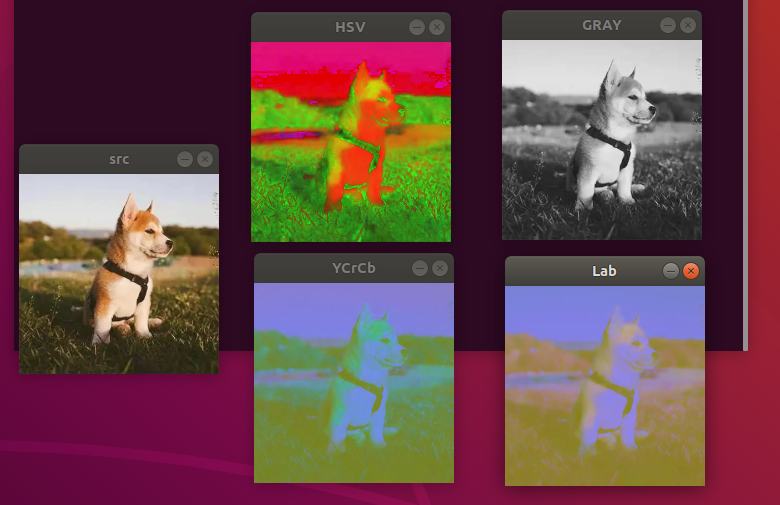
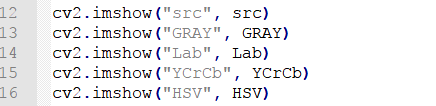
After execution, the final processed result is as follow.
3. Program Analysis
Firstly, import the required module with import statement.
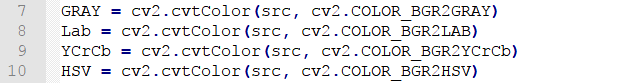
Call imread() function in cv2 module to read the image to be processed.

Next, set the size of the inserted picture. And in the bracket is the name of the picture.

Create four functions in sequence to convert the image into Gray, Lab, Ycrcb amd HSV respectively.
Display the image before and after conversion respectively.
Lastly, close the window through the function.
cv2.waitKey() is a keyboard binding function. Its time unit is milliseconds (ms). The function will wait n ms set in bracket to check if there is any keyboard input. If there is, the ASCII value of the key is returned. -1 will be returned if there is no keyboard input. Generally we set it to 0, the function will wait for keyboard input endlessly.
cv2.destroyAllWindows() is used to delete the window. If there is no parameter in the bracket, all the windows will be deleted. If you input the specific value of the window, the designated window will be removed.
6.2.8 Image Processing — Geometric Transformation
Introduction
A spatial transformation of an image is a geometric transformation of the image coordinate system. It map the coordinate of a picture to a new coordinate of other picture. And geometric transformation will not change the pixel of the image, but rearrange the pixels on the image plane.
According to OpenCV functions, we divide mapping into scaling, flipping,affine transformation, perspective, etc.
Scaling
Scaling is to adjust the size of the picture, for example zoom in or zoom out the picture. In OpenCV, cv2.resize() function is used to scale the image.
dst = cv2.resize(src, dsize[, fx[, fy[, interpolation] ] ] )
dst represents the output image whose type is the same as src. And its size is dsize (when it is not 0) or can be calculated through src.size(), fx and fy.
src represents the original picture
dsize stands for the size of the output image
fx indicates the horizontal scaling ratio
fy denotes the vertical scaling ratio
interpolation is for interpolation method.
| Type | Description |
| cv2.INTER_NEAREST | nearest neighbor interpolation |
| cv2.INTER_LINEAR | linear interpolation |
| cv2.INTER_CUBIC | Cubic spline interpolation. First, the cubic spline fitting is performed on the 4 x 4 nearest neighbors near the original image, and then the cubic spline value corresponding to the target pixel is taken as the value of the corresponding pixel in the target image. |
| cv2.INTER_AREA | Area interpolation similar to nearest interpolation. Sample the current pixel according to the pixels in the surrounding area of the current pixel. |
| cv2.INTER_LANCZOS4 | Lanczos interpolation over 8×8 neighborhood |
| cv2.INTER_LINEAR_EXACT | Bit accurate bilinear interpolation |
| cv2.INTER_MAX | Difference encoding mask |
| cv2.WARP_FILL_OUTLIERS | Flag, fills all of the destination image pixels. If some of them correspond to outliers in the source image, they are set to zero |
| cv2.WARP_INVERSE_MAP | flag, inverse transformation. For example, polar transformation. If flag is not set, perform transformation: dst(ρ,ϕ)=src(x,y) For example, If flag is set, perform transformation: dst(x,y)=src(ρ,ϕ) |
1. Operation Steps
The program will scale the image.
Before operation, please copy the routine “Scale” in “6.2OpenCV->6.2.9Image Processing — Geometric Transformation->Routine Code” to the shared folder.
Note
The input command should be case sensitive and the keywords can be complemented by “Tab” key.
Open virtual machine and start the system. Click “
 ”, and then “
 ” or press “Ctrl+Alt+T” to open command line terminal.
Input command “cd /mnt/hgfs/Share/Scale” and press Enter to enter the shared folder.
cd /mnt/hgfs/Share/Scale
Input command “python3 Scale.py” and press Enter to run the code.
python3 Scale.py
2. Program Outcome
The final output picture is as follow.
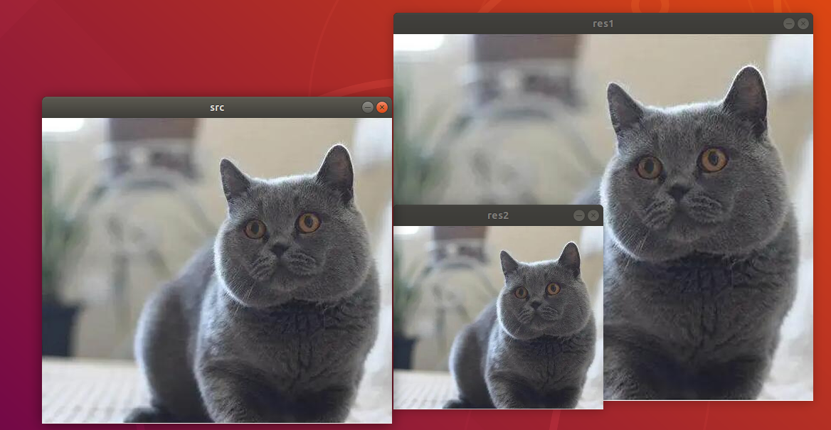
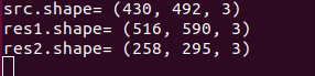
src: Original picture. Its size is 492*430 pixels (width*height)res1: The size of the picture after zoomed in. Its size is 590*512 pixels (width*height)res2: The size of the picture after zoomed out. And its size is 295*258 pixels(width*height)
3. Program Analysis
The routine “Scale.py” can be found in “6. OpenCV Computer Vision Lesson->6.2 Basic Course->6.2.8 Image Processing—Geometric Transformation->Routine Code->Scale.py”.
import numpy as np
import cv2 as cv
src = cv.imread('1.jpg')
# method output the dimension directly
height, width = src.shape[:2] # acquire the original dimension
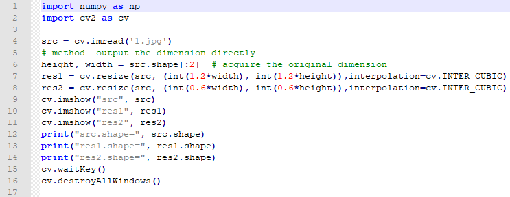
res1 = cv.resize(src, (int(1.2*width), int(1.2*height)),interpolation=cv.INTER_CUBIC)
res2 = cv.resize(src, (int(0.6*width), int(0.6*height)),interpolation=cv.INTER_CUBIC)
cv.imshow("src", src)
cv.imshow("res1", res1)
cv.imshow("res2", res2)
print("src.shape=", src.shape)
print("res1.shape=", res1.shape)
print("res2.shape=", res2.shape)
cv.waitKey()
cv.destroyAllWindows()
Firstly, import the required module through import statement.
import numpy as np
import cv2 as cv
Then call imread() function in cv2 module to read the image that needs to be scaled.
src = cv.imread('1.jpg')
In the bracket is the name of image.
The original width of the picture is 492 pixel, and height is 430 pixel. Parameter dsize can be used to designate the size of target image res1 and res2 (The name of the image can be customized)
The first parameter in dsize corresponds to the width after scaling. (width i.e. the number of columns which is related to parameter fx.) And the second parameter corresponds to the height after scaling. (height i.e. the number of row which is related to parameter fy)
If the value of dsize is specified, the size of the target image is determined by dsize regardless of whether the parameters fx and fy are specified.
height, width = src.shape[:2]  # acquire the original dimension
res1 = cv.resize(src, (int(1.2*width),int(1.2*height)),interpolation=cv.INTER_CUBIC)
res2 = cv.resize(src, (int(0.6*width),int(0.6*height)),interpolation=cv.INTER_CUBIC)
Therefore, program to acquire the original dimension first, and then directly scale the width and height. To zoom in this picture, this routine enlarges the width of res1 to 1.2 times the original and height to 1.2 times the original. Through calculation, the width is 590 pixels (92x1.2) and the height is 516 pixels (430x1.2).
To zoom out the picture, this routine will shrink the res2 width to 0.6 times the original, and the height to 0.6 times the original. The final width is 295 pixels (492x0.6) and height is 258 pixels (430x0.6). And the image size, before and after processing, can printed.
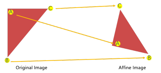
Affine Transformation
Affine transformation is that images can be translated, rotated, etc. through a series of geometric transformations, while lines and parallelism can be preserved.
Linearity means that the straight lines of the image can still be preserved after affine transformation. And parallelism indicates that parallel lines can be preserved after affine transformation.
Translation and rotation are special cases of affine transformation which is realized by the function cv2.warpAffine() in OpenCV. This function execute transformation by a transformation matrix M (transformation matrix of translation and rotation is different)

As the picture below shown, the original image O can be transformed into affine image R by a transformation matrix M.
The format of cv2.warpAffine() function is as follow.
dst = cv2.warpAffine( src, M, dsize[, flags[, borderMode[, borderValue]]] )
dst: Represent the output image after affine transformation. The type of this image is similar to that of the original image. And the actual size of the output image is finally determined by dsize.src: Represent the original imageM: Stand for a 2x3 transformation matrix. Various affine transformation can be realized by using different transformation matrix. And the size of the output image is finally determined by dsize.flags: Represents the interpolation method which defaults to INTER_LINEAR. When it isWARP_INVERSE_MAP, M is an inverse transformation from the target image dst to the original image src.borderMode, optional parameter, represents the edge type,BORDER_CONSTANTby default. When it isBORDER_TRANSPARENT, the values in the target image do not change, and these values correspond to the outliers in the original image.borderValue: Refer to border value, 0 by default.
The optional parameters of cv2.warpAffine() function can be omitted, and its final format is as follow.
dst = cv2.warpAffine( src , M , dsize )
By transformation matrix M, transform the original image src into the target image dst.

Therefore, the type of affine transformation relies on the transformation matrix M.
1. Translation
Translation is the movement of the object. If the coordinates of the object translation is obtained, the following transformation matrix can be created.
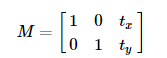
Put the transformation matrix into the array whose type is np.float32, and assign M matrix to cv2.warpAffine() function so as to realize translation.
(1) Operation Steps
This routine will translate the image to right.
Before operation, please copy the routine code in “6. OpenCV Computer Vision Course->6.2 Basic Course->6.2.8 Image Processing — Geometric Transformation->Routine Code” to the shared folder.
The input command should be case sensitive and the keywords can be complemented by “Tab” key.
Open virtual machine and start the system. Click “
”, and then “” or press “Ctrl+Alt+T” to open command line terminal.Input command “cd /mnt/hgfs/Share/Translation/” and press Enter to enter the shared folder.
cd /mnt/hgfs/Share/Translation/
Input command “python3 Translation.py” and press Enter to run the routine.
python3 Translation.py
(2) Program Outcome
The final output picture is as follow.
(3) Program Analysis
The routine “Translation.py” can be found in “6. OpenCV Computer Vision Lesson->6.2 Basic Course->6.2.8 Image Processing—Geometric Transformation->Routine Code->TranslaTion”.
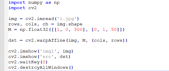
import numpy as np
import cv2

img = cv2.imread('1.jpg')
rows, cols, ch = img.shape
M = np.float32([[1, 0, 300], [0, 1, 50]])

dst = cv2.warpAffine(img, M, (cols, rows))

cv2.imshow('img1', img)
cv2.imshow('src', dst)
cv2.waitKey(0)
cv2.destroyAllWindows()
Firstly, import the required module through import statement.
import numpy as np
import cv2
Then call imread() function in cv2 module to read the image that needs to be translated.
img = cv2.imread('1.jpg')
Return the number of row, column and channel of the image pixel to rows, cols and ch.
rows, cols, ch = img.shape
As mentioned before, if the coordinate of the object translation can be obtained, the transformation matrix can be created.
M = np.float32([[1, 0, 300], [0, 1, 50]])
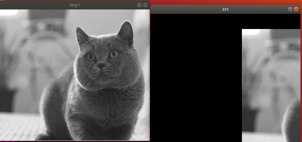
After setting, the picture before and after translation can be displayed through imshow function.
cv2.imshow('img1', img)
cv2.imshow('src', dst)
Lastly, close the window through the function, and you can press any key to exit the program.
cv2.waitKey(0)
cv2.destroyAllWindows()
cv2.waitKey() is a keyboard binding function. Its time unit is milliseconds (ms). The function will wait n ms set in bracket to check if there is any keyboard input. If there is, the ASCII value of the key is returned. -1 will be returned if there is no keyboard input. Generally we set it to 0, the function will wait for keyboard input endlessly.
cv2.destroyAllWindows() is used to delete the window. If there is no parameter in the bracket, all the windows will be deleted. If you input the specific value of the window, the designated window will be removed.
2. Rotation
Both translation and rotation are the examples of the affine transformation, and employ cv2.warpAffine function to realize affine transformation. But their transformation matrix is different. When rotating the image with function cv2.warpAffine(), obtain the transformation matrix with function cv2.getRotationMatrix2D().
The function format is
retval=cv2.getRotationMatrix2D(center, angle, scale)
center refers to the center of rotation.
angle stands for rotation angle. When it is positive, the image will be rotated counterclockwise. When it is negative, the image will be rotated clockwise.
scale means scaled size
The rotation angle θ can be obtained from matrix M.
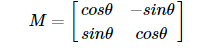
OpenCV has improved this matrix to provide scaling rotation and adjustable rotation center, as the picture shown below.
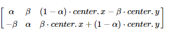
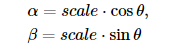
The above matrix represents a rotation around center.x and center.y by θ degrees.
For example, set the function as below to rotate the image around the image center counterclockwise by 45 degree, and zoom out the image 0.6 times the original. Then call this function to generate the matrix.
M=cv2.getRotationMatrix2D((height/2,width/2),45,0.6)
(1) Operation Steps
This routine will rotate the image 90 degree counterclockwise.
Before operation, please copy the routine “Revolve” in “6. OpenCV Computer Vision Course->6.2 Basic Course->6.2.8 Image Processing — Geometric Transformation->Routine Code” to the shared folder.
Note
The input command should be case sensitive and the keywords can be complemented by “Tab” key.
Open virtual machine and start the system. Click “
”, and then “” or press “Ctrl+Alt+T” to open command line terminal.Input command “cd /mnt/hgfs/Share/Revolve/” and press Enter to enter the shared folder.
cd /mnt/hgfs/Share/Revolve/
Input the command “python3 Revolve.py” and press Enter to run the routine.
python3 Revolve.py
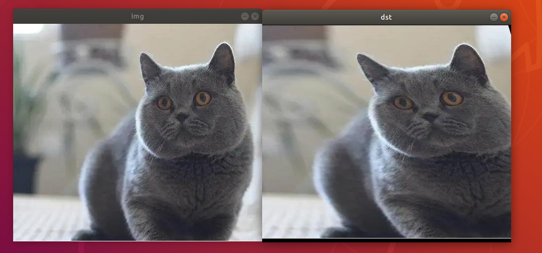
(2) Program Outcome
The output picture is as follow.
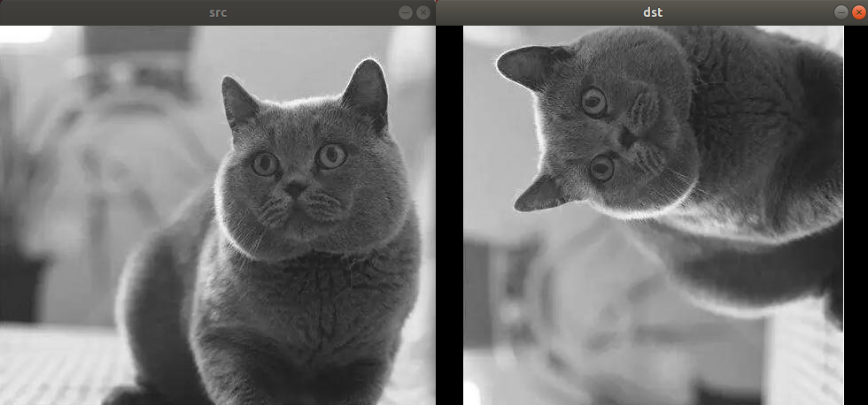
(3) Program Analysis
The routine “Revolve.py” can be found in “6. OpenCV Computer Vision Course->6.2 Basic Course->6.2.8 Image Processing—Geometric Transformation->Routine Code->Revolve”.
import cv2
import numpy as np

img = cv2.imread('1.jpg')
rows, cols, ch = img.shape
# rotate the center  rotation angle  scale factor
M = cv2.getRotationMatrix2D(((cols-1) / 2.0,(rows-1)/2.0), 90,1)
# original picture  convert matrix  output the image center
dst = cv2.warpAffine(img, M, (cols, rows))

cv2.imshow('img', img)
cv2.imshow('dst', dst)
cv2.waitKey(0)
cv2.destroyAllWindows()
Firstly, import the required module through import statement.
import cv2
import numpy as np
Then call
imread()function in cv2 module to read the image that needs to be rotated.
img = cv2.imread('1.jpg')
Return the number of row, column and channel of the image pixel to rows, cols and ch.
rows, cols, ch = img.shape
The image will rotate around the image center 90 degree counterclockwise. And its size remains the same.
M = cv2.getRotationMatrix2D(((cols-1) / 2.0,(rows-1)/2.0), 90,1)
Output the original image center
dst = cv2.warpAffine(img, M, (cols, rows))
After setting, we can call imshow function to display the pictures before and after rotation.
cv2.imshow('img', img)
cv2.imshow('dst', dst)
Lastly, call function below to close the window, and you can press any key to exit the program.
cv2.waitKey(0)
cv2.destroyAllWindows()
cv2.waitKey() is a keyboard binding function. Its time unit is milliseconds (ms). The function will wait n ms set in bracket to check if there is any keyboard input. If there is, the ASCII value of the key is returned. -1 will be returned if there is no keyboard input. Generally we set it to 0, the function will wait for keyboard input endlessly.
cv2.destroyAllWindows() is used to delete the window. If there is no parameter in the bracket, all the windows will be deleted. If you input the specific value of the window, the designated window will be removed.
Perspective Transformation
Affine transformation are rotation, translation and scaling in 2D space, while perspective transformation is in 3D space.
Perspective transformation is realized by function cv2.warpPerspective(), and the function format is as follow.
dst = cv2.warpPerspective( src, M, dsize[, flags[, borderMode[, borderValue]]] )
dst represents the output image after perspective transformation, whose type is the same as the original picture. And its size is determined by dsize.
src represents the image to be processed.
M stands for a 3x3 transformation matrix
dsize indicates the dimension of the output image.
flags represents the interpolation method which defaults to INTER_LINEAR. When it is
WARP_INVERSE_MAP, M is an inverse transformation from the target image dst to the original image src.borderMode, optional parameter, represents the edge type,BORDER_CONSTANTby default. When it isBORDER_TRANSPARENT, the values in the target image do not change, and these values correspond to the outliers in the original image.
1. Operation Steps
This routine will perform perspective transformation.
Before operation, please copy the routine “Perspective” in “6. OpenCV Computer Vision Course->6.2 Basic Course->6.2.8 Image Processing — Geometric Transformation->Routine Code” to the shared folder.
Note
The input command should be case sensitive and the keywords can be complemented by “Tab” key.
Open virtual machine and start the system. Click “
”, and then “” or press “Ctrl+Alt+T” to open command line terminal.Input command “cd /mnt/hgfs/Share/Perspective/” and press Enter to enter the shared folder.
cd /mnt/hgfs/Share/Perspective/
Input command “python3 Perspective.py” and press Enter to run the routine.
python3 Perspective.py
2. Program Outcome
The final output picture is as follow.
3. Program Analysis
The routine “Perspective.py” can be found in “6. OpenCV Computer Vision Course->6.2 Basic Course->6.2.8 Image Processing—Geometric Transformation->Routine Code->Perspective”.
import cv2
import numpy as np

img=cv2.imread('1.jpg')
rows, cols = img.shape[:2]
print(rows,cols)

pts1 = np.float32([[150,50],[400,50],[60,450],[310,450]])
pts2 = np.float32([[50,50],[rows-50,50],[50,cols-50],[rows-50,cols-50]])
M = cv2.getPerspectiveTransform(pts1,pts2)
dst = cv2.warpPerspective(img,M,(cols,rows))

cv2.imshow("img",img)
cv2.imshow("dst",dst)
cv2.waitKey()
cv2.destroyAllWindows()
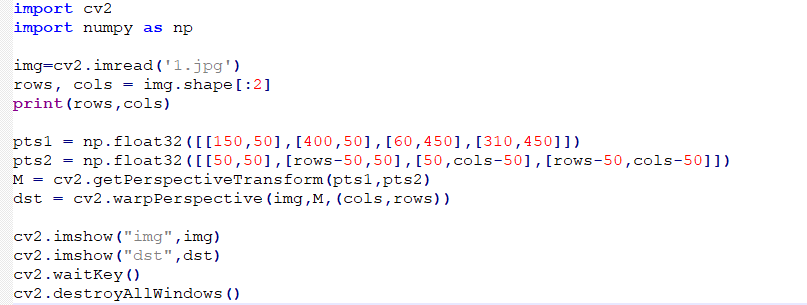
Firstly, import the required module through import statement.
import cv2
import numpy as np
Then call imread() function in cv2 module to read the image for perspective transformation.
img=cv2.imread('1.jpg')
Return the number of row, column and channel of the image pixel to rows, cols and ch.
rows, cols = img.shape[:2]
In this example, specify four vertices pts1 of the parallelogram in the original image, and specify four vertices pts2 of the rectangle in the target image. Next, generate the transformation matrix M with dst=cv2.warpPerspective(img,M,(cols,rows)). Next, employ dst=cv2.warpPerspective(img,M,(cols,rows)) statement to convert parallelogram to rectangle.
pts1 = np.float32([[150,50],[400,50],[60,450],[310,450]])
pts2 = np.float32([[50,50],[rows-50,50],[50,cols-50],[rows-50,cols-50]])
M = cv2.getPerspectiveTransform(pts1,pts2)
dst = cv2.warpPerspective(img,M,(cols,rows))
After setting, the picture before and after translation can be displayed through imshow function.
cv2.imshow("img",img)
cv2.imshow("dst",dst)
Lastly, close the window through the function, and you can press any key to exit the program.
cv2.waitKey()
cv2.destroyAllWindows()
cv2.waitKey() is a keyboard binding function. Its time unit is milliseconds (ms). The function will wait n ms set in bracket to check if there is any keyboard input. If there is, the ASCII value of the key is returned. -1 will be returned if there is no keyboard input. Generally we set it to 0, the function will wait for keyboard input endlessly.
cv2.destroyAllWindows() is used to delete the window. If there is no parameter in the bracket, all the windows will be deleted. If you input the specific value of the window, the designated window will be removed.
Remap
Remap is that the pixels are mapped from one picture to the corresponding positions in another image according to the rules to form a new image.
As the pixel coordinates of the original image do not correspond to that of target image, in general, we describe the position (x, y) of each pixel by remapping.
g(x,y)=f(h(x,y))
g() refers to target image, f() is the original image and h(x,y) is the image after remapping. Take the below function for example. And image I will be remapped under the following conditions.
h(x,y)=(I.cols-x,y)
The image will flip in the x direction. cv2.remap() function in OpenCV makes it more convenient and free to remap. And its format is as follow.
dst = cv2.remap( src, map1, map2, interpolation\[, borderMode\[, borderValue\]\] )
dst represents the output image whose type and size are the same as the original picture.
src represents the original image
There are two possible values of map1 parameter. It represents a map of (x,y), or x value of (x,y) of CV_16SC2 , CV_32FC1, CV_32FC2 type.
There are also two possible values of map2 parameter.
When map1 represents (x,y), its value is none.
When map1 represents x value of (x,y), its value is the y value of (x,y) in CV_16UC1, CV_32FC1 type.
Note
map1 refers to the column where the pixel is located, and map2 refers to the row where the pixel is located. So usually, map1 is written as mapx and map2 as mapy for better understanding.
Interpolation is for interpolation method.
borderMode refers to border value. When it is BORDER_TRANSPARENT, the pixel of target image corresponding to outliers in the original image will not be modified.
borderValue refers to border value, 0 by default.
1. Copy Pixel
(1) Operation Steps
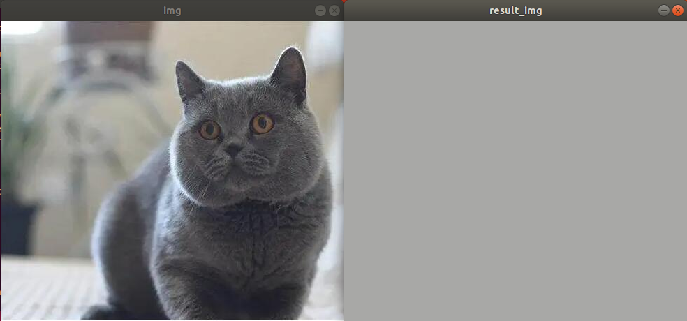
All pixels in the target image are mapped to the pixels on the 100th row and 200th column in the original image.
Before operation, please copy the routine “Remap” in “6. OpenCV Computer Vision Course->6.2 Basic Course->6.2.8 Image Processing — Geometric Transformation->Routine Code” to the shared folder.
Note
The input command should be case sensitive and the keywords can be complemented by “Tab” key.
Open virtual machine and start the system. Click “
”, and then “” or press “Ctrl+Alt+T” to open command line terminal.Input command “cd /mnt/hgfs/Share/Remap/” and press Enter to enter the shared folder.
cd /mnt/hgfs/Share/Remap/
Input command “python3 copy.py” and press Enter to run the routine.
python3 copy.py
(2) Program Outcome
A pure-colored picture will be output.
(3) Program Analysis
The routine “copy.py” can be found in “6. OpenCV Computer Vision Course->6.2 Basic Course->6.2.8 Image Processing—Geometric Transformation->Routine Code->Remap”.
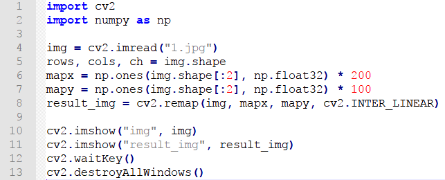
import cv2
import numpy as np

img = cv2.imread("1.jpg")
rows, cols, ch = img.shape
mapx = np.ones(img.shape[:2], np.float32) * 200
mapy = np.ones(img.shape[:2], np.float32) * 100
result_img = cv2.remap(img, mapx, mapy, cv2.INTER_LINEAR)

cv2.imshow("img", img)
cv2.imshow("result_img", result_img)
cv2.waitKey()
cv2.destroyAllWindows()
Firstly, import the required module through import statement.
import cv2
import numpy as np
Then call
imread()function in cv2 module to read the image that needs to be scaled.
img = cv2.imread("1.jpg")
Return the number of row, column and channel of the image pixel to rows, cols and ch.
rows, cols, ch = img.shape
mapx and mapy separately set the x axis and y axis coordinate. Map all the pixels on the target image to the pixels on 100th row, 200th column of the original image.
mapx = np.ones(img.shape[:2], np.float32) * 200
mapy = np.ones(img.shape[:2], np.float32) * 100
After setting, the picture before and after the pixels are copied can be displayed through imshow function. Lastly, close the window through the function, and you can press any key to exit the program.
cv2.imshow("img", img)
cv2.imshow("result_img", result_img)
cv2.waitKey()
cv2.destroyAllWindows()
cv2.waitKey() is a keyboard binding function. Its time unit is milliseconds (ms). The function will wait n ms set in bracket to check if there is any keyboard input. If there is, the ASCII value of the key is returned. -1 will be returned if there is no keyboard input. Generally we set it to 0, the function will wait for keyboard input endlessly.
cv2.destroyAllWindows() is used to delete the window. If there is no parameter in the bracket, all the windows will be deleted. If you input the specific value of the window, the designated window will be removed.
2. Copy the Whole Image
(1) Operation Steps
Besides the pixels can be copied, the whole image can also be copied. For example, copy the whole original picture to the right.
Before operation, please copy the routine “Remap” in “6. OpenCV Computer Vision Course->6.2 Basic Course->6.2.8 Image Processing — Geometric Transformation->Routine Code” to the shared folder.
Note
The input command should be case sensitive and the keywords can be complemented by “Tab” key.
Open virtual machine and start the system. Click “
”, and then “” or press “Ctrl+Alt+T” to open command line terminal.Input command “cd /mnt/hgfs/Share/Remap/” and press Enter to enter the shared folder.
cd /mnt/hgfs/Share/Remap/
Input command “python3 copy_all.py” and press Enter to run the routine.
python3 copy_all.py

(2) Program Outcome
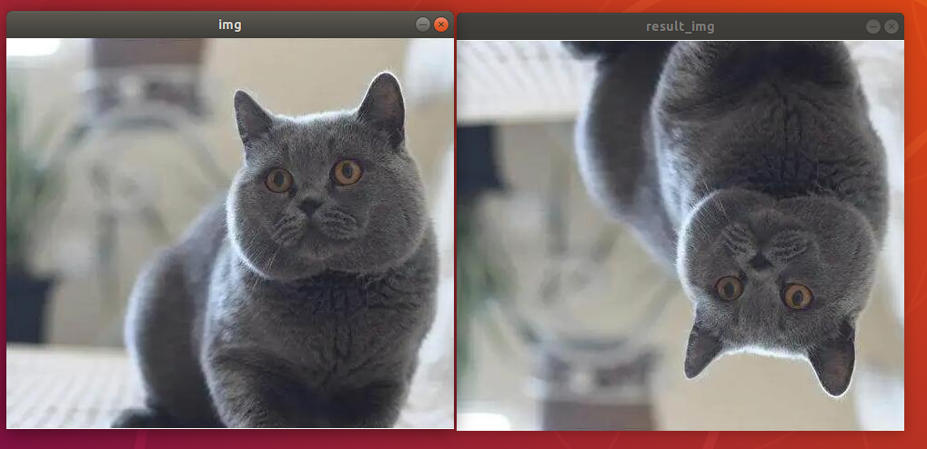
Correspond all the pixels of the original image to those of original image. The final output image is as follow.
(3) Program Analysis
The routine “copy_all.py” can be found in “6. OpenCV Computer Vision Course->6.2 Basic Course->6.2.8 Image Processing—Geometric Transformation->Routine Code”.
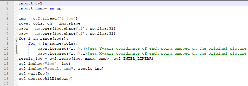
import cv2
import numpy as np

img = cv2.imread("1.jpg")
rows, cols, ch = img.shape
mapx = np.ones(img.shape[:2], np.float32)
mapy = np.ones(img.shape[:2], np.float32)
for i in range(rows):
    for j in range(cols):
        mapx.itemset((i,j),j)#set Y-axis coordinate of each point mapped on the original picture
        mapy.itemset((i,j),i)#set X-axis coordinate of each point mapped on the original picture
result_img = cv2.remap(img, mapx, mapy, cv2.INTER_LINEAR)
cv2.imshow("img", img)
cv2.imshow("result_img", result_img)
cv2.waitKey()
cv2.destroyAllWindows()
Firstly, import the required module through import statement.
import cv2
import numpy as np
Then call
imread()function in cv2 module to read the image.
img = cv2.imread("1.jpg")
Return the number of row, column and channel of the image pixel to rows, cols and ch.
rows, cols, ch = img.shape
mapx and mapy separately set the x axis and y axis coordinate.
mapx = np.ones(img.shape[:2], np.float32)
mapy = np.ones(img.shape[:2], np.float32)
for i in range(rows):
    for j in range(cols):
        mapx.itemset((i,j),j)#set Y-axis coordinate of each point mapped on the original picture
        mapy.itemset((i,j),i)#set X-axis coordinate of each point mapped on the original picture
After setting, the picture before and after the pixels are copied can be displayed through imshow function. Lastly, close the window through the function, and you can press any key to exit the program.
cv2.imshow("img", img)
cv2.imshow("result_img", result_img)
cv2.waitKey()
cv2.destroyAllWindows()
cv2.waitKey() is a keyboard binding function. Its time unit is milliseconds (ms). The function will wait n ms set in bracket to check if there is any keyboard input. If there is, the ASCII value of the key is returned. -1 will be returned if there is no keyboard input. Generally we set it to 0, the function will wait for keyboard input endlessly.
cv2.destroyAllWindows() is used to delete the window. If there is no parameter in the bracket, all the windows will be deleted. If you input the specific value of the window, the designated window will be removed.
3. Rotate Around X Axis
If make the image flip around x axis,
x axis coordinate remains unchanged.
The y-axis coordinate after rotation is symmetric with respect to x axis.
Or:
map1 remains unchanged
map2= total number of row - 1 - current row number
(1) Operation Steps
With cv2.remap() function, the pixels can be remapped, and also be flipped and then remapped. Ensure the x axis coordinate remains unchanged and y-axis coordinate after rotation is symmetric with respect to x axis.
Before operation, please copy the routine “Remap” in “6. OpenCV Computer Vision Course->6.2 Basic Course->6.2.8 Image Processing — Geometric Transformation->Routine Code” to the shared folder.
Note
The input command should be case sensitive and the keywords can be complemented by “Tab” key.
Open virtual machine and start the system. Click “
”, and then “” or press “Ctrl+Alt+T” to open command line terminal.Input the command “cd /mnt/hgfs/Share/Remap/” and press Enter to enter the shared folder.
cd /mnt/hgfs/Share/Remap/
Input command “python3 x_rotation.py” and press Enter to run the routine.
python3 x_rotation.py

(2) Program Outcome
The final output image is as follow.
(3) Program Analysis
The routine “x_rotation.py” can be found in “6. OpenCV Computer Vision Course->6.2 Basic Course->6.2.8 Image Processing—Geometric Transformation->Routine Code”.
import cv2
import numpy as np

img = cv2.imread("1.jpg")
rows, cols, ch = img.shape
mapx = np.ones(img.shape[:2], np.float32)
mapy = np.ones(img.shape[:2], np.float32)
for i in range(rows):
    for j in range(cols):
        mapx.itemset((i,j),j)
        mapy.itemset((i,j),rows-1-i)#just modify this line of code. Symmetrical

result_img = cv2.remap(img, mapx, mapy, cv2.INTER_LINEAR)
cv2.imshow("img", img)
cv2.imshow("result_img", result_img)
cv2.waitKey()
cv2.destroyAllWindows()
Firstly, import the required module through import statement.
import cv2
import numpy as np
Then call
imread()function in cv2 module to read the image that needs to be scaled.
img = cv2.imread("1.jpg")
Return the number of row, column and channel of the image pixel to rows, cols and ch.
rows, cols, ch = img.shape
mapx and mapy separately set the x axis and y axis coordinate. map1 remains unchanged, and map2 = “total number of row - 1 - current row number”
After setting, the picture before and after can be displayed through imshow function. Lastly, close the window through the function, and you can press any key to exit the program.
cv2.imshow("img", img)
cv2.imshow("result_img", result_img)
cv2.waitKey()
cv2.destroyAllWindows()
cv2.waitKey() is a keyboard binding function. Its time unit is milliseconds (ms). The function will wait n ms set in bracket to check if there is any keyboard input. If there is, the ASCII value of the key is returned. -1 will be returned if there is no keyboard input. Generally we set it to 0, the function will wait for keyboard input endlessly.
cv2.destroyAllWindows() is used to delete the window. If there is no parameter in the bracket, all the windows will be deleted. If you input the specific value of the window, the designated window will be removed.
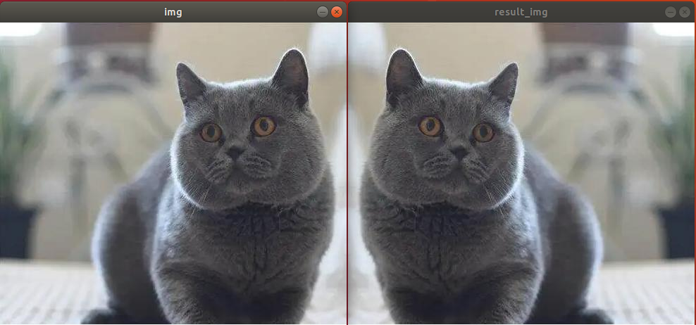
4. Rotate Around Y Axis
If make the image flip around y axis,
y axis coordinate remains unchanged.
The x-axis coordinate after rotation is symmetric with respect to y axis.
Or:
Map2 remains unchanged
map2 = “total number of column - 1 - current column number”
(1) Operation Steps
Before operation, please copy the routine “Remap” in “6. OpenCV Computer Vision Course->6.2 Basic Course->6.2.8 Image Processing — Geometric Transformation->Routine Code” to the shared folder.
Note
The input command should be case sensitive and the keywords can be complemented by “Tab” key.
Open virtual machine and start the system. Click “
”, and then “” or press “Ctrl+Alt+T” to open command line terminal.Input command “cd /mnt/hgfs/Share/Remap/” and press Enter to enter the shared folder.
cd /mnt/hgfs/Share/Remap/
Input command “python3 copy_all.py” and press Enter to run the routine.
python3 copy_all.py

(2) Program Outcome
The final output image is as follow.
(3) Program Analysis
The routine “y_rotation.py” can be found in “6. OpenCV Computer Vision Course->6.2 Basic Course->6.2.8 Image Processing—Geometric Transformation->Routine Code”.
import cv2
import numpy as np
img = cv2.imread("1.jpg")
rows, cols, ch = img.shape
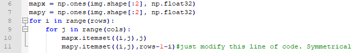
mapx = np.ones(img.shape[:2], np.float32)
mapy = np.ones(img.shape[:2], np.float32)
for i in range(rows):
for j in range(cols):
mapx.itemset((i,j),cols-1-j)#just modify this line of code.
mapy.itemset((i,j),i)#
result_img = cv2.remap(img, mapx, mapy, cv2.INTER_LINEAR)
cv2.imshow("img", img)
cv2.imshow("result_img", result_img)
cv2.waitKey()
cv2.destroyAllWindows()
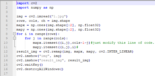
Firstly, import the required module through import statement.
import cv2
import numpy as np
Then call
imread()function in cv2 module to read the image that needs to be scaled.
img = cv2.imread("1.jpg")
Return the number of row, column and channel of the image pixel to rows, cols and ch.
rows, cols, ch = img.shape
mapx and mapy separately set the x axis and y axis coordinate. mapy remains unchanged, and mapx = “total number of column - 1 - current column number”
mapx = np.ones(img.shape[:2], np.float32)
mapy = np.ones(img.shape[:2], np.float32)
for i in range(rows):
    for j in range(cols):
        mapx.itemset((i,j),cols-1-j)#just modify this line of code.
        mapy.itemset((i,j),i)#
After setting, the picture before and after can be displayed through imshow function. Lastly, close the window through the function, and you can press any key to exit the program.
cv2.imshow("img", img)
cv2.imshow("result_img", result_img)
cv2.waitKey()
cv2.destroyAllWindows()
cv2.waitKey() is a keyboard binding function. Its time unit is milliseconds (ms). The function will wait n ms set in bracket to check if there is any keyboard input. If there is, the ASCII value of the key is returned. -1 will be returned if there is no keyboard input. Generally we set it to 0, the function will wait for keyboard input endlessly.
cv2.destroyAllWindows() is used to delete the window. If there is no parameter in the bracket, all the windows will be deleted. If you input the specific value of the window, the designated window will be removed.
5. Rotate Around XY Axis
If make the image rotate around x axis and y axis,
The x-axis coordinate after rotation is symmetric with respect to y axis.
The y-axis coordinate after rotation is symmetric with respect to x axis.
Or:
map1 = “total number of row - 1 - current row number”
map2= “total number of row - 1 - current row number”
(1) Operation Steps
Before operation, please copy the routine “Remap” in “6. OpenCV Computer Vision Course->6.2 Basic Course->6.2.8 Image Processing — Geometric Transformation->Routine Code” to the shared folder.
Note
The input command should be case sensitive and the keywords can be complemented by “Tab” key.
Open virtual machine and start the system. Click “
”, and then “” or press “Ctrl+Alt+T” to open command line terminal.Input command “cd /mnt/hgfs/Share/Remap/” and press Enter to enter the shared folder.
cd /mnt/hgfs/Share/Remap/
Input command “python3 xy_rotation.py” and press Enter to run the routine.
python3 xy_rotation.py
(2) Program Outcome
The final output picture is as follow.
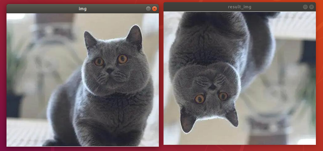
(3) Program Analysis
The routine “xy_rotation.py” can be found in “6. OpenCV Computer Vision Course->6.2 Basic Course->6.2.8 Image Processing—Geometric Transformation->Routine Code”.
import cv2
import numpy as np

img = cv2.imread("1.jpg")
rows, cols, ch = img.shape
mapx = np.ones(img.shape[:2], np.float32)
mapy = np.ones(img.shape[:2], np.float32)
for i in range(rows):
    for j in range(cols):
        mapx.itemset((i,j),cols-1-j)
        mapy.itemset((i,j),rows-1-i)
result_img = cv2.remap(img, mapx, mapy, cv2.INTER_LINEAR)
cv2.imshow("img", img)
cv2.imshow("result_img", result_img)
cv2.waitKey()
cv2.destroyAllWindows()
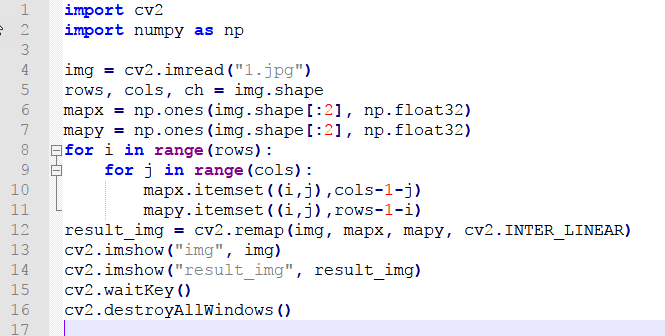
Firstly, import the required module through import statement.
import cv2
import numpy as np
Then call
imread()function in cv2 module to read the image that needs to be scaled.
img = cv2.imread("1.jpg")
Return the number of row, column and channel of the image pixel to rows, cols and ch.
rows, cols, ch = img.shape
mapx and mapy separately set the x axis and y axis coordinate. The value of mapy is changed as “total number of row - 1 - current row number”, and mapx = “total number of column - 1 - current column number”
mapx = np.ones(img.shape[:2], np.float32)
mapy = np.ones(img.shape[:2], np.float32)
for i in range(rows):
    for j in range(cols):
        mapx.itemset((i,j),cols-1-j)
        mapy.itemset((i,j),rows-1-i)
After setting, the picture before and after can be displayed through imshow function. Lastly, close the window through the function, and you can press any key to exit the program.
cv2.imshow("img", img)
cv2.imshow("result_img", result_img)
cv2.waitKey()
cv2.destroyAllWindows()
cv2.waitKey() is a keyboard binding function. Its time unit is milliseconds (ms). The function will wait n ms set in bracket to check if there is any keyboard input. If there is, the ASCII value of the key is returned. -1 will be returned if there is no keyboard input. Generally we set it to 0, the function will wait for keyboard input endlessly.
cv2.destroyAllWindows() is used to delete the window. If there is no parameter in the bracket, all the windows will be deleted. If you input the specific value of the window, the designated window will be removed.
6. Compress Image
Compressing image is to compress the original image by half.
(1) Operation Steps
Before operation, please copy the routine “Scale” in “6. OpenCV Computer Vision Course->6.2 Basic Course->6.2.8 Image Processing — Geometric Transformation->Routine Code” to the shared folder.
Note
The input command should be case sensitive and the keywords can be complemented by “Tab” key.
Open virtual machine and start the system. Click “
”, and then “” or press “Ctrl+Alt+T” to open command line terminal.Input command “cd /mnt/hgfs/Share/Remap/” and press Enter to enter the shared folder.
cd /mnt/hgfs/Share/Remap/
Input command “python3 half_size.py” and press Enter to run the code.
python3 half_size.py
(2) Program Outcome
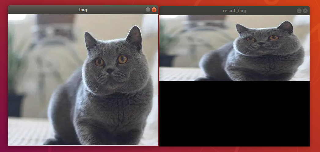
(3) Program Analysis
The routine “half_size.py” can be found in “6. OpenCV Computer Vision Course->6.2 Basic Course->6.2.8 Image Processing—Geometric Transformation->Routine Code”.
import cv2
import numpy as np

img = cv2.imread("1.jpg")
rows, cols, ch = img.shape
mapx = np.ones(img.shape[:2], np.float32)
mapy = np.ones(img.shape[:2], np.float32)
for i in range(rows):
    for j in range(cols):
        mapx.itemset((i,j),j)
        mapy.itemset((i,j),2*i)#just modify this line of code
result_img = cv2.remap(img, mapx, mapy, cv2.INTER_LINEAR)
cv2.imshow("img", img)
cv2.imshow("result_img", result_img)
cv2.waitKey()
cv2.destroyAllWindows()
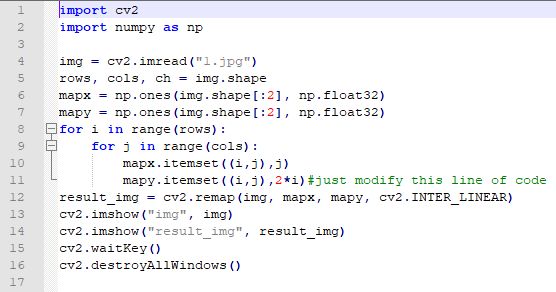
Firstly, import the required module through import statement.
import cv2
import numpy as np
Then call
imread()function in cv2 module to read the image.
img = cv2.imread("1.jpg")
Return the number of row, column and channel of the image pixel to rows, cols and ch.
rows, cols, ch = img.shape
mapx and mapy separately set the x axis and y axis coordinate and double the X axis
mapx = np.ones(img.shape[:2], np.float32)
mapy = np.ones(img.shape[:2], np.float32)
for i in range(rows):
    for j in range(cols):
        mapx.itemset((i,j),j)
        mapy.itemset((i,j),2*i)#just modify this line of code
After setting, the picture before and after can be displayed through imshow function. Lastly, close the window through the function, and you can press any key to exit the program
cv2.imshow("img", img)
cv2.imshow("result_img", result_img)
cv2.waitKey()
cv2.destroyAllWindows()
cv2.waitKey() is a keyboard binding function. Its time unit is milliseconds (ms). The function will wait n ms set in bracket to check if there is any keyboard input. If there is, the ASCII value of the key is returned. -1 will be returned if there is no keyboard input. Generally we set it to 0, the function will wait for keyboard input endlessly.
cv2.destroyAllWindows() is used to delete the window. If there is no parameter in the bracket, all the windows will be deleted. If you input the specific value of the window, the designated window will be removed.
6.2.9 Image Processing - Smoothing
Image Noise
During collecting, processing and transferring, the digital image will be disturbed by different noises, which leads to low-quality image, obscure image and disappeared image feature. And image smoothing is to improve the image by removing noise, and salt-and-pepper noise as well as Gauss noise are common.
1. Salt-and-pepper Noise
Salt-and-pepper noise is also known as pulse noise which is white dots and black dots appearing randomly, like there are black pixels in bright area and white pixels in dark area.
At left is the original picture and the right is the picture with salt-and-pepper noise.
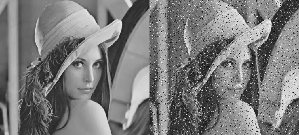
2. Gauss Noise
Gauss noise is a term from signal processing theory denoting a kind of signal noise that has a probability density function (pdf) equal to that of the normal distribution (which is also known as the Gaussian distribution). Commonly, it can be suppressed by mathematical statistics.
At left is the original picture and the right is the picture with Gauss noise.
Image Smoothing
From the perspective of signal, image smoothing is to filter the high frequency part of the signal and reserve the low frequency part.
Based on filter, filtering can be divided into mean filtering, Gaussian filtering and median filtering.
1. Mean Filtering
The idea of mean filtering is simply to take the mean of all the pixels of the image that is assign the mean of all the pixels in the unit of a square to the center pixel.
Take the picture below as example. In picture (a), the center pixel value is “226” and the mean of all the pixels is “122” obtained from the equation below, and “122” is the new center pixel value.
Replace the original center pixel value by “122” as the picture (b) shown.
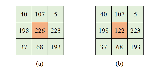
The algorithm of the mean filtering is simple and its calculation speed is fast. However, the details of the image are destroyed during removing noise resulting in low definition.
2. Gauss Filtering
The weighted mean is calculated by multiplying each value by the corresponding weight, adding the sum, and then dividing the sum by the number of the values.
Gauss filtering is to obtain the weighted mean of all the pixels of the image that is assign the weighted mean in the unit of a square to the center pixel.
Take the picture below as example. In picture (a), the center pixel value is “226” and the weighted mean of all the pixels is “164” obtained from the equation below, and “164” is the new center pixel value. $\( 40\times 0.05 + 107 \times 0.1 + 5 \times 0.05 + 198 \times 0.1 + 226 \times 0.4 + 223 \times 0.1 + 37 \times 0.05 + 68 \times 0.1 + 193 \times 0.05= 164 \)$ Replace the original center pixel value by “122” as the picture (c) shown.
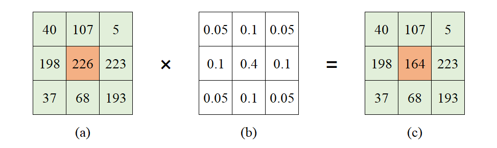
3. Median Filtering
The median is the middle value when a data set is ordered from least to greatest.
Median filtering is to take the median of all the pixels of the image that is assign the median in the unit of square to the center pixel.
Take the picture below as example. In picture (a), the center pixel value is “226” and the medium of the pixels is “107”, and “107” is the new center pixel value.
Replace the original center pixel value by “107” as the picture (b) shown.
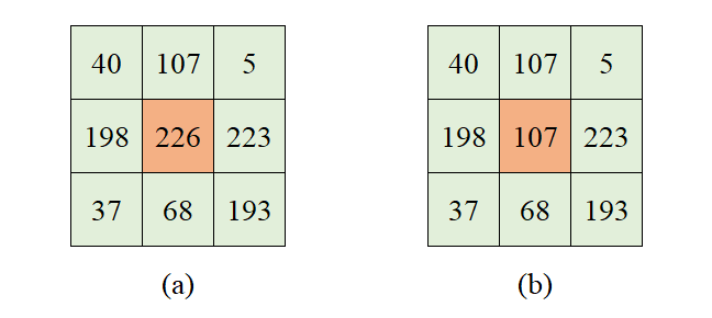
Operation Steps
This routine will execute mean filtering, Gauss filtering and median filtering separately.
Before operation, please copy the routine “filtering.py” in “6. OpenCV Computer Vision Course->6.2 Basic Course->6.2.9 Image Processing — Smoothing->Routine Code” to the shared folder.
Note
The input command should be case sensitive and the keywords can be complemented by “Tab” key.
Open virtual machine and start the system. Click “
 ”, and then “
 ” or press “Ctrl+Alt+T” to open command line terminal.
Input command “cd /mnt/hgfs/Share/” and press Enter to enter the shared folder.
cd /mnt/hgfs/Share/
Input command “python3 filtering.py” and press Enter to run the routine.
python3 filtering.py
Program Outcome
The final output image is as follow.
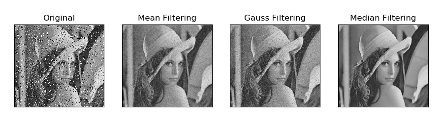
Program Analysis
The routine “filtering.py” can be found in “6. OpenCV Computer Vision Course->6.2 Basic Course->6.2.9 Image Processing — Smoothing->Routine Code”.
import cv2
import numpy as np
import matplotlib.pyplot as plt

# image reading
img = cv2.imread('noise.jpg')

# image smoothing
blur1 = cv2.blur(img, (5, 5))   # mean filtering
blur2 = cv2.GaussianBlur(img, (5, 5), 1)    # Gauss filtering
blur3 = cv2.medianBlur(img, 5)  # Median filtering

# image display
plt.figure(figsize=(10, 5), dpi=100)
plt.rcParams['axes.unicode_minus'] = False
plt.subplot(141), plt.imshow(img), plt.title("Original")
plt.xticks([]), plt.yticks([])
plt.subplot(142), plt.imshow(blur1), plt.title("Mean Filtering")
plt.xticks([]), plt.yticks([])
plt.subplot(143), plt.imshow(blur2), plt.title("Gauss Filtering")
plt.xticks([]), plt.yticks([])
plt.subplot(144), plt.imshow(blur3), plt.title("Median Filtering")
plt.xticks([]), plt.yticks([])
plt.show()
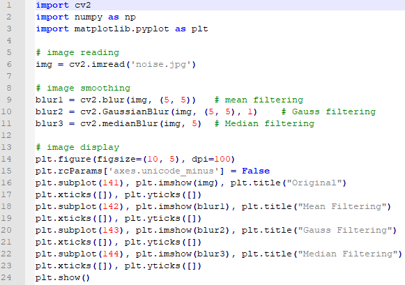
1. Image Processing
(1) Import Module
Firstly, import the required module through import statement.
import cv2
import numpy as np
import matplotlib.pyplot as plt
(2) Read Images
Then call imread() function in cv2 module to read the image that needs to be filtered.
img = cv2.imread('noise.jpg')
In the bracket is the image name.
(3) Mean Filtering
Call blur() function in cv2 module to perform mean filtering on the specific image.
blur1 = cv2.blur(img, (5, 5)) # mean filtering
The format of blur() function is as follow.
cv2.blur(scr, ksize)
The first parameter scr is the input image.
The second parameter ksize is the size of convolution kernel.
(4) Gauss Filtering
Call GaussianBlur() function in cv2 module to perform Gauss filtering on the specific image.
blur2 = cv2.GaussianBlur(img, (5, 5), 1) # Gauss filtering
The format of GaussianBlur() function is as follow.
cv2.GaussianBlur(src, ksize, sigmaX, sigmaY, borderType)
The first parameter scr is the input image.
The second parameter ksize is the size of Gaussian convolution kernel. Both the height and width of the convolution kernel must be positive number and odd number.
The third parameter sigmaX is the horizontal standard deviation of Gaussian kernel.
The fourth parameter sigmaY is the vertical standard deviation of Gaussian kernel, 0 by default.
The fifth parameter borderType is the type of border filling.
(5) Median Filtering
Call medianBlur() function in cv2 module to perform median filtering on the specific image.
blur3 = cv2.medianBlur(img, 5) # Median filtering
The format of medianBlur() function is as follow
cv2.medianBlur(src, ksize)
The first parameter scr is the input image.
The second parameter ksize is the size of the convolution kernel.
2. Image Display
(1) Create Custom Image
Call figure() function in matplotlib.pyplot module to create a custom image for displaying the final output image.
plt.figure(figsize=(10, 5), dpi=100)
The format of the figure() function is as follow.
matplotlib.pyplot.figure(num=None, figsize=None, dpi=None, facecolor=None, edgecolor=None, frameon=True, FigureClass=<class 'matplotlib.figure.Figure'>, clear=False, **kwargs)
The first parameter num is the only identifier of the image i.e. the serial number of the picture (number) or the name (string).
The second parameter figsize is the width and height of the image in inch.
The third parameter dpi is the resolution of the image i.e. the number of pixels by inch
The fourth parameter facecolor is the background color.
The fifth parameter edgecolor is the frame color
The sixth parameter frameon determines whether to draw the picture, and it is True by default.
The seventh parameter FigureClass is used to select the custom figure when generating the image
The eighth parameter clear determines whether to clear all the original images.
The ninth parameter **kwargs represents other properties of the image.
(2) Modify matplotlib Configuration
matplotlib is plotting library of Python. User can access and modify matplotlib configuration options through parameter dictionary rcParams.
plt.rcParams['axes.unicode_minus'] = False
The codes above are used to manipulate the display of the normal characters.
(3) Set the Parameter of Image Display
Call subplot(), imshow() and title() functions in matplotlib.pyplot modules to designate the position, color and headline of the subplot in the Figure.
plt.subplot(141), plt.imshow(img), plt.title("Original")
subplot() function is used to set the position of the subplot, and the function format is as follow.
matplotlib.pyplot.subplot(nrows, ncols, index, **kwargs)
The first parameter nrows and the second parameter ncols respectively are the number of row and column of subplot.
The third parameter index is the index position. Index starts at 1 in the upper left corner and increases to the right.
When both the row and column are less than “10”, these two values can be abbreviated to an integer. For example, the meaning of subplot(1, 4, 1) and subplot(141) are the same, both representing the image is divided into one row and four columns, and the subplot is in the first place i.e. 1st row, 1st column.
imshow() function is used to set the color of subplot, and its format is as follow.
matplotlib.pyplot.imshow(X, cmap=None)
The first parameter “X” is the image data.
The second parameter cmap is the colormap, RGB(A) color space by default.
title()function is used to set the title of the subplot. The parameter in the bracket is the name of the subplot and the function format is as follow.
matplotlib.pyplot.title(label, fontdict=None, loc=None, pad=None, *, y=None, **kwargs)
The first parameter label is the title composed of string.
The second parameter fontdict is the property of the font, and the current parameter refers to dictionary.
The third parameter loc is the position of the title. It can be left, center or right, and center by default.
The fourth parameter pad is the padding distance (inside margin) between the tile and the subplot, “6.0” by default.
The fifth parameter “y” is the vertical distance between the title and the subplot, and the unit is the percentage of the height of the subplot. The default value is “None”, that is, the position of the title is automatically determined to avoid overlapping with other elements. “1.0” means the title is at the top of the subplot.
The sixth parameter **kwargs is the text object keyword property, which is used to determine the appearance of the text, such as font, text color, etc.
(4) Set Axis Tick
Call xticks() and yticks() function in matplotlib.pyplot module to set the tick and tag of X and Y axis. As the coordinate axis is not required in image display in this routine, the list is set as none that is the coordinate axis will not be displayed.
plt.xticks([]), plt.yticks([])
The format of xticks() function is as follow.
xticks(ticks=None, labels=None, **kwargs)
When the parameter is none, the function will return the current tick and tag of X axis. Otherwise the function is used to set the current tick and label of X axis.
The first parameter ticks is a list of the positions of the X-axis ticks. If the list is empty, the X-axis ticks will be cleared.
The second parameter labels is the label of X-axis tick. Only when parameter “ticks” is not none, can this parameter be passed.
The third parameter **kwargs is used to control the appearance of the tick and label.
The format of yticks() is the same as that of xticks(). The difference lies in the controlled object.
(5) Display Image
Call show() function in matplotlib.pyplot module to display the image on the window.
plt.show()
The complete codes of image display part are as follow.
plt.figure(figsize=(10, 5), dpi=100)
plt.rcParams['axes.unicode_minus'] = False
plt.subplot(141), plt.imshow(img), plt.title("Original")
plt.xticks([]), plt.yticks([])
plt.subplot(142), plt.imshow(blur1), plt.title("Mean Filtering")
plt.xticks([]), plt.yticks([])
plt.subplot(143), plt.imshow(blur2), plt.title("Gauss Filtering")
plt.xticks([]), plt.yticks([])
plt.subplot(144), plt.imshow(blur3), plt.title("Median Filtering")
plt.xticks([]), plt.yticks([])
plt.show()
6.2.10 Image Processing—Edge Detection
Edge Detection Introduction
Edge detection is fundamental technique in image processing and computer vision, which aims at identifying edges in a digital image at which the image brightness changes sharply. Sharp changes in image usually reflect important events and changes in properties. The edge is as the picture shown.
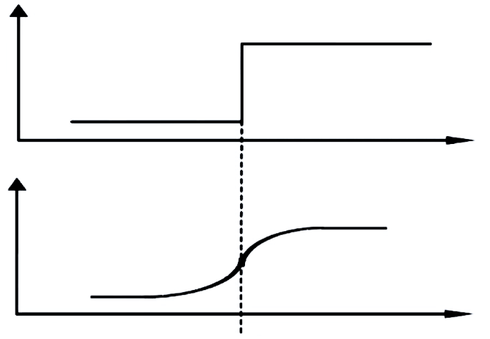
Edge detection greatly reduces the amount of data, removes irrelevant information, and preserves the important structural properties of the image. Edge detection is divided into two types.
Based on search: The boundary is detected by finding the maximum and minimum values in the first derivative of the image, and it usually locates in the direction with the largest gradient. The representative algorithms are the Sobel operator and the Scharr operator.
Based on zero-crossing: the boundary is found by searching the second-order derivative zero-crossing of the image, which is usually the Laplacian zero-crossing point or the zero-crossing point represented by the nonlinear difference, and the representative algorithm is the Laplacian operator.
Canny Edge Detection
Canny Edge Detection is a popular edge detection algorithm. It was developed by John F. Canny in 1986 and considered as the best algorithm of edge detection. Canny edge detection will go through 4 steps, including Noise Reduction, Finding Gradient Magnitude and Direction of the Image, Non-maximum Suppression and Hysteresis Thresholding.
1. Noise Reduction
Since edge detection is susceptible to noise in the image, first step is to remove the noise in the image. For detailed operation, please refer to the file in “6. OpenCV Computer Vision Course->6.2 Basic Course->6.2.9 Image Processing—Smoothing”.
2. Finding Gradient Magnitude and Direction of the Image
In math, gradient is a vector, indicating that the directional derivative of the function at a certain point reaches the maximum along this direction, that is, the function changes the fastest along the direction at this point, and the rate of change is the greatest.
In the image, gradient represents the degree and direction of gray value change, and the edge refers to the position where the gray intensity changes the most. Gradient direction is always perpendicular to edges.
Sobel filter is used to calculate the magnitude and direction of the gradient. The Sobel operator GX is the first derivative in the horizontal direction, which is used to detect the edge in the Y-axis direction, while GY is the the first derivative in the vertical direction, which is used to detect the edge in the X-axis direction.
The formula for calculating the gradient size is as follows $\( G = \ \sqrt{(G_{X}^{2} + G_{Y}^{2})} \)\( The formula for calculating the gradient direction is as follows \)\( \theta = arctan\frac{G_{Y}}{G_{X}} \)$
3. Non-Maximum Suppression
Non-Maximum Suppression (NMS) is that reserve local maximum and suppress all the values apart from local maximum. In simple terms, all the pixels of the image will be detected. If the gradient intensity of a point is greater than the pixels in the positive and negative directions of its gradient direction, the point is retained; otherwise, the point is suppressed.
Canny edge detection algorithm perform non-maximum suppression along the gradient direction not the edge direction.
4. Hysteresis Thresholding
This stage decides which are really edges. For this, we need two threshold values, “minVal” and “maxVal”. Any edges with intensity gradient more than maxVal are sure to be edges and those below minVal are sure to be non-edges. Those who lie between these two thresholds are classified edges or non-edges based on their connectivity. If they are connected to “sure-edge” pixels, they are considered to be part of edges. Otherwise, they are also discarded.
Operation Steps
This routine will perform the edge detection.
Before operation, please copy the routine “edge_detection.py”and sample picture “luna.jpg” in “6. OpenCV Computer Vision Course->6.2 Basic Course->6.2.10 Image Processing—Edge Detection->Routine Code” to the shared folder.
Note
The input command should be case sensitive and the keywords can be complemented by “Tab” key.
Open virtual machine and start the system. Click “
 ”, and then “
 ” or press “Ctrl+Alt+T” to open command line terminal.
Input command “cd /mnt/hgfs/Share/” and press Enter to enter the shared folder.
cd /mnt/hgfs/Share/
Input command “python3 edge_detection.py” and press Enter to run the routine.
python3 edge_detection.py
Program Outcome
The final output image is as follow.
Program Analysis
The routine “edge_detection.py” can be found in “6. OpenCV Computer Vision Course->6.2 Basic Course->6.2.10 Image Processing—Edge Detection->Routine Code”.
import cv2
import numpy as np
import matplotlib.pyplot as plt

# read the image
img = cv2.imread('luna.jpg')

# Canny edge detection
lowThreshold = 1
max_lowThreshold = 80
canny = cv2.Canny(img, lowThreshold, max_lowThreshold)

# image display
plt.figure(figsize=(8, 5), dpi=100)
plt.rcParams['axes.unicode_minus'] = False
plt.subplot(121), plt.imshow(img, cmap=plt.cm.gray), plt.title("Original")
plt.xticks([]), plt.yticks([])
plt.subplot(122), plt.imshow(canny, cmap=plt.cm.gray), plt.title("Edge Detection")
plt.xticks([]), plt.yticks([])
plt.show()
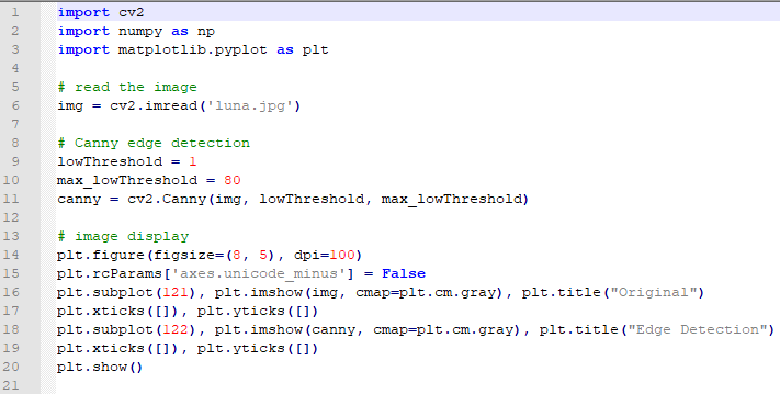
1. Image Processing
(1) Import Module
Firstly, import the required module through import statement.
import cv2
import numpy as np
import matplotlib.pyplot as plt
(2) Read Image
Call imread() function in cv2 module to read the image
img = cv2.imread('luna.jpg')
The parameter in the bracket is the name of the image.
(3) Set Threshold
Set two thresholds to determine the final edge.
lowThreshold = 1
max_lowThreshold = 80
(4) Edge Detection
Call Canny() function in cv2 module to perform edge detection on the specific image.
canny = cv2.Canny(img, lowThreshold, max_lowThreshold)
The format of Canny() function is as follow.
Canny( image, threshold1, threshold2)
The first parameter image is the input image.
The second parameter threshold1 is the low threshold minVal
The third parameter threshold2 is high threshold maxVal.
2. Image Display
(1) Create Custom Figure
Call figure() function in matplotlib.pyplot module to create a custom figure for displaying the final output image.
plt.figure(figsize=(8, 5), dpi=100)
The format of the figure() function is as follow.
figure(num=None, figsize=None, dpi=None, facecolor=None, edgecolor=None, frameon=True, FigureClass=<class 'matplotlib.figure.Figure'>, clear=False, **kwargs)
The first parameter num is the only identifier of the image i.e. the serial number of the picture (number) or the name (string).
The second parameter figsize is the width and height of the image in inch.
The third parameter dpi is the resolution of the image i.e. the number of pixels by inch
The fourth parameter facecolor is the background color.
The fifth parameter edgecolor is the frame color
The sixth parameter frameon determines whether to draw the picture, and it is “True” by default.
The seventh parameter FigureClass is used to select the custom figure when generating the image
The eighth parameter clear determines whether to clear all the original images.
The ninth parameter **kwargs represents other properties of the image.
(2) Modify matplotlib Configuration
matplotlib is plotting library of Python. User can access and modify matplotlib configuration options through parameter dictionary rcParams.
plt.rcParams['axes.unicode_minus'] = False
The codes above are used to manipulate the display of the normal characters.
(3) Set the Parameter of Image Display
Call subplot(), imshow() and title() functions in matplotlib.pyplot modules to designate the position, color and headline of the subplot in the Figure.
plt.subplot(121), plt.imshow(img, cmap=plt.cm.gray), plt.title("Original")
subplot() function is used to set the position of the subplot, and the function format is as follow.
subplot(nrows, ncols, index, **kwargs)
The first parameter nrows and the second parameter ncols respectively are the number of row and column of subplot.
The third parameter index is the index position. Index starts at 1 in the upper left corner and increases to the right.
When both the row and column are less than “10”, these two values can be abbreviated to an integer. For example, the meaning of subplot(1, 2, 1) and subplot(121) are the same, both representing the image is divided into one row and 2 columns, and the subplot is in the first place i.e. 1st row, 1st column.
imshow()function is used to set the color of subplot, and its format is as follow.
imshow(X, cmap=None)
The first parameter “X” is the image data.
The second parameter cmap is the colormap, RGB(A) color space by default.
title()function is used to set the title of the subplot. The parameter in the bracket is the name of the subplot and the function format is as follow.
title(label, fontdict=None, loc=None, pad=None, *, y=None, **kwargs)
The first parameter label is the title composed of string.
The second parameter fontdict is the property of the font, and the current parameter refers to dictionary.
The third parameter loc is the position of the title. It can be left, center or right, and center by default.
The fourth parameter pad is the padding distance (inside margin) between the tile and the subplot, “6.0” by default.
The fifth parameter “y” is the vertical distance between the title and the subplot, and the unit is the percentage of the height of the subplot. The default value is “None”, that is, the position of the title is automatically determined to avoid overlapping with other elements. “1.0” means the title is at the top of the subplot.
The sixth parameter **kwargs is the text object keyword property, which is used to determine the appearance of the text, such as font, text color, etc.
(4) Set Axis Tick
Call xticks() and yticks() function in matplotlib.pyplot module to set the tick and tag of X and Y axis. As the coordinate axis is not required in image display in this routine, the list is set as none that is the coordinate axis will not be displayed.
plt.xticks([]), plt.yticks([])
The format of xticks() function is as follow.
xticks(ticks=None, labels=None, **kwargs)
When the parameter is none, the function will return the current tick and tag of X axis. Otherwise the function is used to set the current tick and label of X axis.
The first parameter ticks is a list of the positions of the X-axis ticks. If the list is empty, the X-axis ticks will be cleared.
The second parameter labels is the label of X-axis tick. Only when parameter “ticks” is not none, can this parameter be passed.
The third parameter **kwargs is used to control the appearance of the tick and label.
The format of yticks() is the same as that of xticks(). The difference lies in the controlled object.
(5) Display Image
Call show() function in matplotlib.pyplot module to display the image on the window.
plt.show()
The complete codes of image display part are as follow.
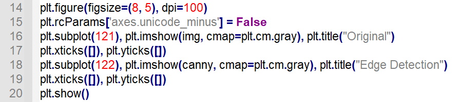
6.2.11 Image Processing — Morphological Processing
Morphology Introduction
Morphology is one of the most widely used techniques in image processing. It is mainly used to extract image components that are meaningful for describing the shape of an area, so that the most essential shape features of the target object can captured in subsequent recognition, such as boundaries and connected areas. In addition, techniques such as thinning, pixelation, and burr trimming are often used in image preprocessing and postprocessing, which can greatly strengthen the image.
The basic idea of morphology is to use a special structural element to measure or extract the corresponding shape or feature in the input image for further image analysis and target recognition.
Morphological Transformation
1. Erosion and Dilation
Both erosion and dilation are the basic and important morphological operation, and also the foundations of multiple advanced morphological processing. Many morphological algorithms are composed of these two.
(1) Structuring Element
Structuring element is required in erosion and dilation. A two-dimensional structuring element can be seen as a two-dimensional matrix element which is “0” or “1”.
(2) Erosion
Erosion works to remove small and meaningless object, and the whole process is divided into three steps.
Build an image matrix upon the structuring element and determine its origin. Take the element at the upper left corner as the origin, and mark it with dark color.
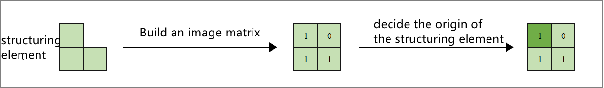
Overlay the structuring element on the pending image. If the value of the pixel in the image corresponding to the elements whose value is “1” in the structuring elements are all “1”, the pixel at the corresponding position of the origin is assigned as “1”, otherwise it is “0”.
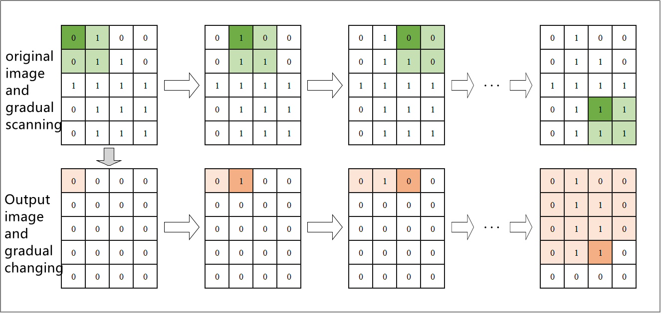
Make the structuring elements move on the pending image in order until all the images are processed completely.
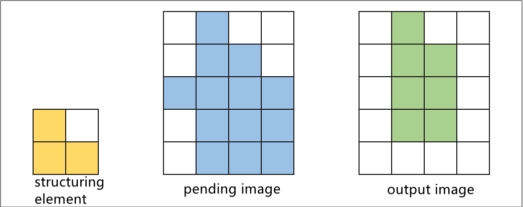
(3) Dilation
Dilation can enlarge the edge of the image and pad the edge of the target object or non-target pixel. The operations are divided into three steps.
Build an image matrix upon the structuring element and determine its origin. Take the element at the upper left corner as the origin, and mark it with dark color.
Overlay the structuring element on the pending image. If at least one of the value of the pixel in the image corresponding to the elements whose value is “1” in the structuring elements is “1”, the pixel at the corresponding position of the origin is assigned as “1”, otherwise it is “0”.
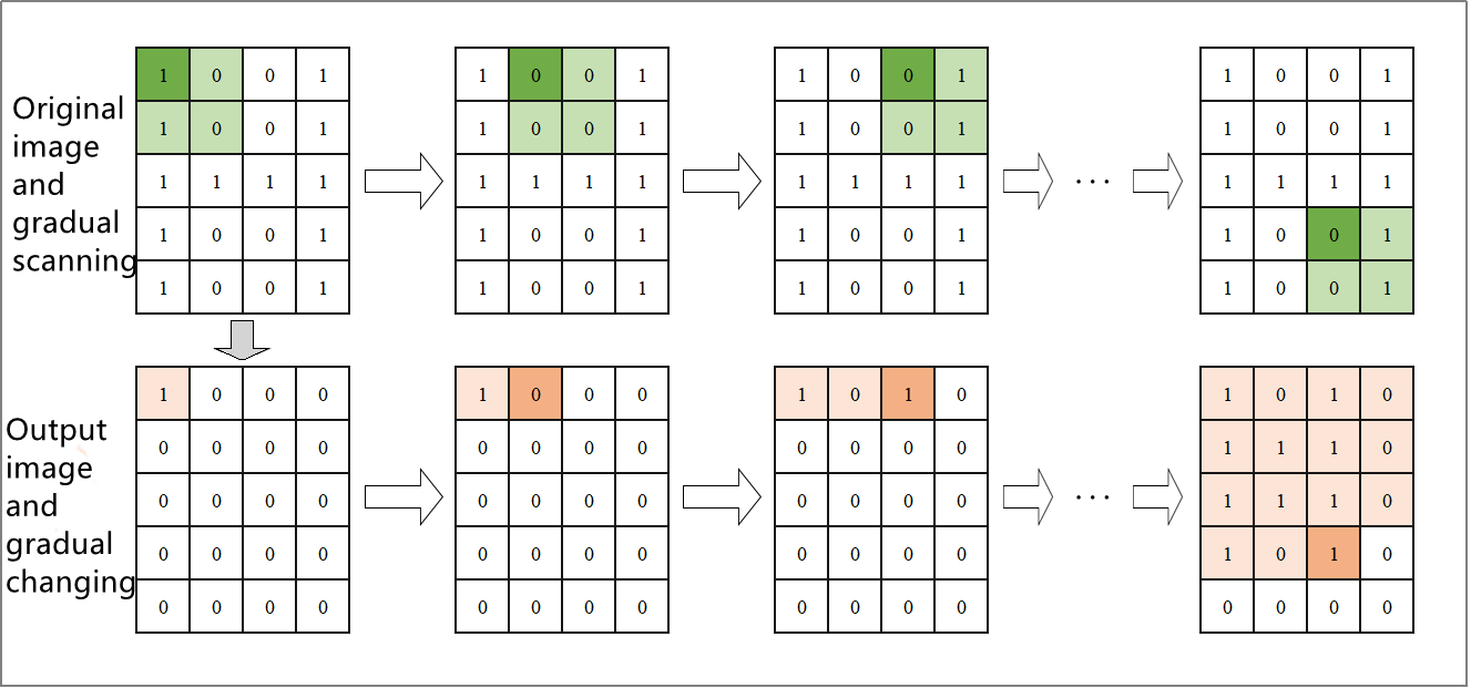
Make the structuring elements move on the pending image in order until all the images are processed completely.
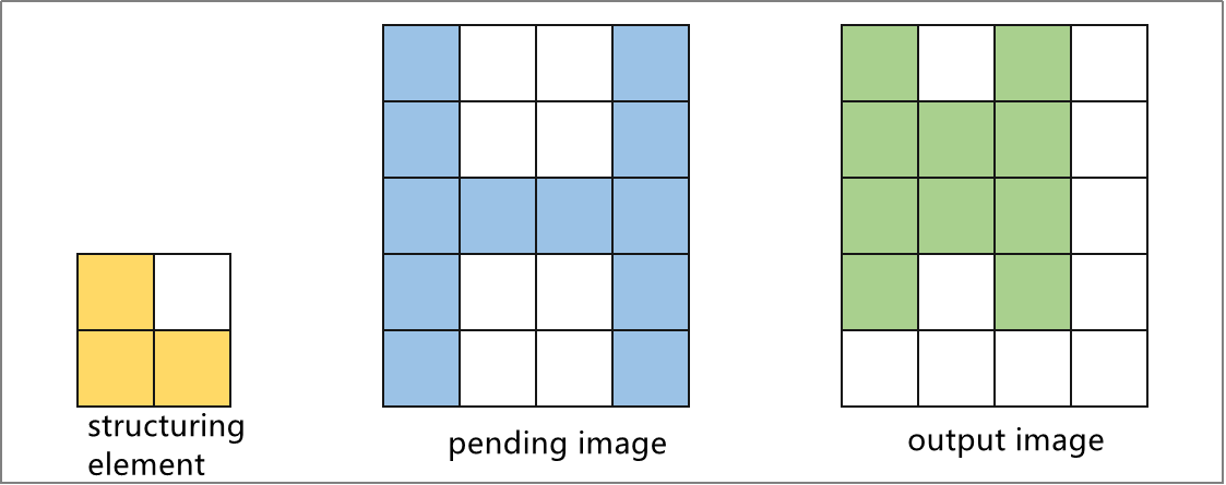
2. Opening and Closing
In opening and closing, erosion and dilation are executed in sequence.
(1) Open Operation
Opening indicates that erosion is executed first and dilation follows. It is useful in separating objects, removing small area, removing highlight under dark background.
(2) Close Operation
In closing, dilation is executed first and erosion follows. It plays an important role in eliminating holes, that is, filling closed areas and deleting dark areas under a bright background.
3. Top Hat and Bottom Hat
(1) Top Hat Operation
It is the difference between input image and the image after opening (Top hat operation= input image - image after opening), and it can obtain areas with brighter gray in the original image
(2) Bottom Hat Operation (Black Hat)
It is the difference between input image and the image after closing (Top hat operation= input image - image after closing), and it can obtain areas with darker gray in the original image
Operation Steps
This routine will perform erosion, dilation, opening, closing, top hat operation and bottom hat operation on the designated image.
Before operation, please copy the routine “example_org.jpg” in “6. OpenCV Computer Vision Course->6.2 Basic Course->6.2.11 Image Processing — Morphological Processing->Routine Code” to the shared folder.
Note
The input command should be case sensitive and the keywords can be complemented by “Tab” key.
Open virtual machine and start the system. Click “
 ”, and then “
 ” or press “Ctrl+Alt+T” to open command line terminal.
Input command “cd /mnt/hgfs/Share/” and press Enter to enter the shared folder.
cd /mnt/hgfs/Share/
Input command “python3 morphology operations.py” and press Enter to run the routine.
python3 morphology operations.py
Program Outcome
The final output image is as follow.
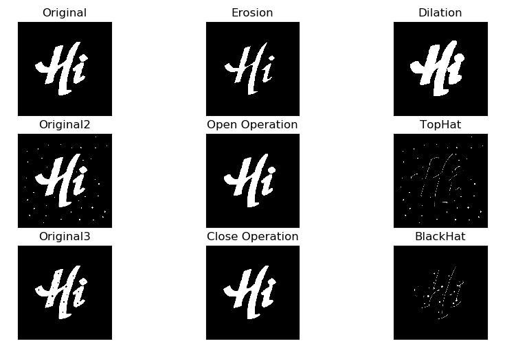
Program Analysis
The routine “morphology_operations.py” can be found in “6. OpenCV Computer Vision Course->6.2 Basic Course->6.2.11 Image Processing—Morphological Processing->Routine Code”.
import cv2
import numpy as np
import matplotlib.pyplot as plt

# read the image
img_org = cv2.imread('example_org.jpg')
img_noise = cv2.imread('example_noise.jpg')
img_cave = cv2.imread('example_cave.jpg')

# build nuclear structure
kernel = np.ones((10, 10), np.uint8)  # 10*10 all-one matrix

# Morphological processing
erosion_img = cv2.erode(img_org, kernel)  # erosion
dilate_img = cv2.dilate(img_org, kernel)  # dilation
open_img = cv2.morphologyEx(img_noise, cv2.MORPH_OPEN, kernel)  # open operation
close_img = cv2.morphologyEx(img_cave, cv2.MORPH_CLOSE, kernel)  # close operation
top_hat_img = cv2.morphologyEx(img_noise, cv2.MORPH_TOPHAT, kernel)  # top hat operation
black_hat_img = cv2.morphologyEx(img_cave, cv2.MORPH_BLACKHAT, kernel)  # bottom hat operation

# image display
plt.figure(figsize=(10, 6), dpi=100)
plt.rcParams['axes.unicode_minus'] = False

plt.subplot(331), plt.imshow(img_org), plt.title("Original")
plt.xticks([]), plt.yticks([])
plt.subplot(332), plt.imshow(erosion_img), plt.title("Erosion")
plt.xticks([]), plt.yticks([])
plt.subplot(333), plt.imshow(dilate_img), plt.title("Dilation")
plt.xticks([]), plt.yticks([])

plt.subplot(334), plt.imshow(img_noise), plt.title("Original2")
plt.xticks([]), plt.yticks([])
plt.subplot(335), plt.imshow(open_img), plt.title("Open Operation")
plt.xticks([]), plt.yticks([])
plt.subplot(336), plt.imshow(top_hat_img), plt.title("TopHat")
plt.xticks([]), plt.yticks([])

plt.subplot(337), plt.imshow(img_cave), plt.title("Original3")
plt.xticks([]), plt.yticks([])
plt.subplot(338), plt.imshow(close_img), plt.title("Close Operation")
plt.xticks([]), plt.yticks([])
plt.subplot(339), plt.imshow(black_hat_img), plt.title("BlackHat")
plt.xticks([]), plt.yticks([])

plt.show()
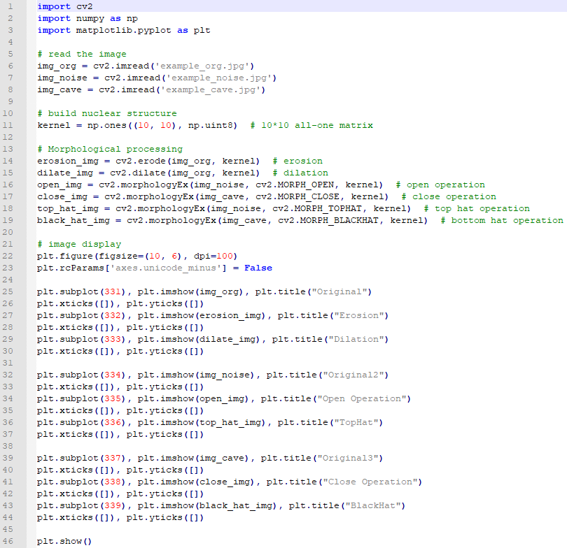
1. Image Processing
(1) Import Module
Firstly, import the required module through import statement.
import cv2
import numpy as np
import matplotlib.pyplot as plt
(2) Read the Image
Then call imread() function in cv2 module to read the pending image.
img_org = cv2.imread('example_org.jpg')
img_noise = cv2.imread('example_noise.jpg')
img_cave = cv2.imread('example_cave.jpg')
The parameter in the bracket is the name of the image
(3) Create Nuclear Structure
Call ones() function in numpy module to create the nuclear structure i.e. array required in the operation.
kernel = np.ones((10, 10), np.uint8) # 10*10 all-one matrix
The format of ones() function is as follow.
np.ones(shape, dtype=None, order='C')
The first parameter shape is a integer or integer tuple used to define the size of the array. If it designates the variable of the integer, one–dimensional array will be returned. If it designate integer tuple, the array in given shape will be returned.
The second parameter dtype refers to the data type of the array, float by default.
The third parameter order is used to designate the storing order of the returned array elements in storage.
(4) Erosion and Dilation
Call erode() and dilate() function in cv2 module to perform erosion and dilation on the specific image.
erosion_img = cv2.erode(img_org, kernel)  # erosion
dilate_img = cv2.dilate(img_org, kernel)  # dilation
The format of erode() function is as follow.
cv2.erode(src, kernel, iteration)
The first parameter src is the input image.
The second parameter kernel is the size of the kernel.
The third parameter is the umber of iteration.
The meaning of the parameter in dilate() function is the same as that of erode() function.
(5) Open Operation and Close Operation
Call morphologyEx() function in cv2 module to perform open operation, close operation, top hat operation and bottom hat operation on the specific image.
open_img = cv2.morphologyEx(img_noise, cv2.MORPH_OPEN, kernel)  # open operation
close_img = cv2.morphologyEx(img_cave, cv2.MORPH_CLOSE, kernel)  # close operation
top_hat_img = cv2.morphologyEx(img_noise, cv2.MORPH_TOPHAT, kernel)  # top hat operation
black_hat_img = cv2.morphologyEx(img_cave, cv2.MORPH_BLACKHAT, kernel)  # bottom hat operation
The format of morphologyEx() function is as follow.
cv2.morphologyEx(img, op, kernel)
The first parameter img indicates the input image
The second parameter oprepresents the operation type.
| Operation Type | Meaning |
|---|---|
| cv2.MORPH_OPEN | open operation |
| cv2.MORPH_CLOSE | close operation |
| cv2.MORPH_GRADIENT | morphological gradient |
| cv2.MORPH_TOPHAT | top hat operation |
| cv2.MORPH_BLACKHAT | bottom hat operation |
The third parameter indicates the size of the frame.
2. Image Display
(1) Create Custom Figure
Call figure() function in matplotlib.pyplot module to create a custom figure for displaying the final output image.
plt.figure(figsize=(10, 6), dpi=100)
The format of the figure() function is as follow.
matplotlib.pyplot.figure(num=None, figsize=None, dpi=None, facecolor=None, edgecolor=None, frameon=True, FigureClass=<class 'matplotlib.figure.Figure'>, clear=False, **kwargs)
The first parameter num is the only identifier of the image i.e. the serial number of the picture (number) or the name (string).
The second parameter figsize is the width and height of the image in inch.
The third parameter dpi is the resolution of the image i.e. the number of pixels by inch
The fourth parameter facecolor is the background color.
The fifth parameter edgecolor is the frame color
The sixth parameter frameon determines whether to draw the picture, and it is True by default.
The seventh parameter FigureClass is used to select the custom figure when generating the image
The eighth parameter clear determines whether to clear all the original images.
The ninth parameter **kwargs represents other properties of the image.
(2) Modify matplotlib Configuration
matplotlib is plotting library of Python. User can access and modify matplotlib configuration options through parameter dictionary rcParams.
plt.rcParams['axes.unicode_minus'] = False
The codes above are used to manipulate the display of the normal characters.
(3) Set the Parameter of Image Display
Call subplot(), imshow() and title() functions in matplotlib.pyplot modules to designate the position, color and headline of the subplot in the Figure.
plt.subplot(331), plt.imshow(img_org), plt.title("Original")
subplot()function is used to set the position of the subplot, and the function format is as follow.
matplotlib.pyplot.subplot(nrows, ncols, index, **kwargs)
The first parameter nrows and the second parameter ncols respectively are the number of row and column of subplot.
The third parameter index is the index position. Index starts at 1 in the upper left corner and increases to the right.
When both the row and column are less than “10”, these two values can be abbreviated to an integer. For example, the meaning of subplot(3, 3, 1) and subplot(331) are the same, both representing the image is divided into three rows and three columns, and the subplot is in the first place i.e. 1st row, 1st column.
imshow() function is used to set the color of subplot, and its format is as follow.
matplotlib.pyplot.imshow(X, cmap=None)
The first parameter X is the image data.
The second parameter cmap is the colormap, RGB(A) color space by default.
title()function is used to set the title of the subplot. The parameter in the bracket is the name of the subplot and the function format is as follow.
matplotlib.pyplot.title(label, fontdict=None, loc=None, pad=None, *, y=None, **kwargs)
The first parameter label is the title composed of string.
The second parameter fontdict is the property of the font, and the current parameter refers to dictionary.
The third parameter loc is the position of the title. It can be left, center or right, and center by default.
The fourth parameter pad is the padding distance (inside margin) between the tile and the subplot, “6.0” by default.
The fifth parameter “y” is the vertical distance between the title and the subplot, and the unit is the percentage of the height of the subplot. The default value is None, that is, the position of the title is automatically determined to avoid overlapping with other elements. “1.0” means the title is at the top of the subplot.
The sixth parameter **kwargs is the text object keyword property, which is used to determine the appearance of the text, such as font, text color, etc.
(4) Set Axis Tick
Call xticks() and yticks() function in matplotlib.pyplot module to set the tick and tag of X and Y axis. As the coordinate axis is not required in image display in this routine, the list is set as none that is the coordinate axis will not be displayed.
plt.xticks([]), plt.yticks([])
The format of xticks() function is as follow.
matplotlib.pyplot.xticks(ticks=None, labels=None, **kwargs)
The first parameterticks is a list of the positions of the X-axis ticks. If the list is empty, the X-axis ticks will be cleared.
The second parameter labels is the label of X-axis tick. Only when parameter “ticks” is not none, can this parameter be passed.
The third parameter **kwargs is used to control the appearance of the tick and label.
The format of yticks() is the same as that of xticks(). The difference lies in the controlled object.
(5) Display Image
Call show() function in matplotlib.pyplot module to display the image on the window.
plt.show()
The complete codes of image display part are as follow.
plt.subplot(331), plt.imshow(img_org), plt.title("Original")
plt.xticks([]), plt.yticks([])
plt.subplot(332), plt.imshow(erosion_img), plt.title("Erosion")
plt.xticks([]), plt.yticks([])
plt.subplot(333), plt.imshow(dilate_img), plt.title("Dilation")
plt.xticks([]), plt.yticks([])

plt.subplot(334), plt.imshow(img_noise), plt.title("Original2")
plt.xticks([]), plt.yticks([])
plt.subplot(335), plt.imshow(open_img), plt.title("Open Operation")
plt.xticks([]), plt.yticks([])
plt.subplot(336), plt.imshow(top_hat_img), plt.title("TopHat")
plt.xticks([]), plt.yticks([])

plt.subplot(337), plt.imshow(img_cave), plt.title("Original3")
plt.xticks([]), plt.yticks([])
plt.subplot(338), plt.imshow(close_img), plt.title("Close Operation")
plt.xticks([]), plt.yticks([])
plt.subplot(339), plt.imshow(black_hat_img), plt.title("BlackHat")
plt.xticks([]), plt.yticks([])

plt.show()
6.2.12 Image Processing — Thresholding
Image Binaryzation
Image binaryzation is to set the gray values of image pixels as two values, 0 (represent black) and 255 (represent white) generally, which will make the image turn black-and-white.
Commonly, it will process the grayscale image, and then set a threshold to divide the image into two parts, including the part greater than the threshold and the part smaller than the threshold. Next, assign different pixel values to these two parts of image.
Image binaryzation facilitates the further processing of the image, makes the image simple, reduces the amount of data and highlights the target contour you are interested in.
Under different situation, there are three ways to execute thresholding, including Global Thresholding, Adaptive Thresholding and Otsu Thresholding
Global Thresholding
Global thresholding will process the whole image according to the set threshold.
1. Operation Steps
Note
Before operation, please copy the routine “threshold_demo.py” and sample picture “test.jpg” in “6. OpenCV Computer Vision Course->6.2 Basic Course->6.2.12 Image Processing — Thresholding->Routine Code” to the shared folder.
The input command should be case sensitive and the keywords can be complemented by “Tab” key.
(1) Open virtual machine and start the system. Click “ ”, and then “
 ” or press “Ctrl+Alt+T” to open command line terminal.
(2) Input command “cd /mnt/hgfs/share/” and press Enter to enter the shared folder.
cd /mnt/hgfs/share/
(3) Input command “python3 threshold_demo.py” and press Enter to run the routine.
python3 threshold_demo.py
2. Program Outcome
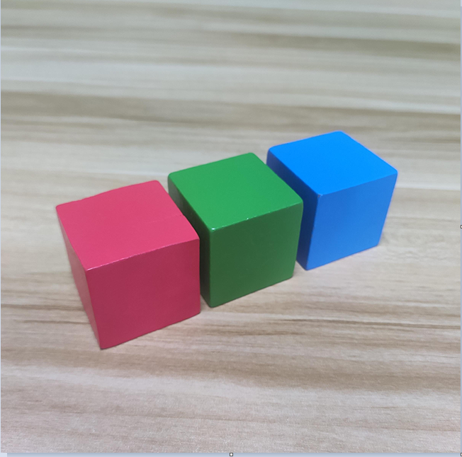
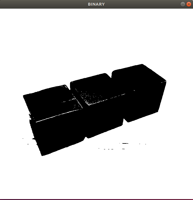
The final output picture is as shown above.
3. Code Analysis
The routine “threshold_demo.py” can be found in “6. OpenCV Computer Vision Course->6.2 Basic Course->6.2.12 Image Processing — Thresholding->Routine Code”.
import cv2
img=cv2.imread('test.jpg')
img_gray = cv2.cvtColor(img,cv2.COLOR_BGR2GRAY)
ret, img2 = cv2.threshold(img_gray, 127, 255, cv2.THRESH_BINARY)
#the threshold is 127
#set maxval as 255. And the output image after processing is black-and-white image
cv2.imshow("BINARY", img2)
cv2.waitKey(0)
cv2.destroyAllWindows()
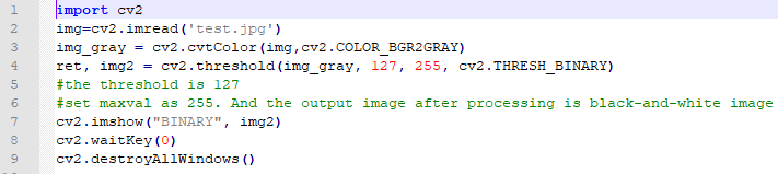
Import Module:Import cv2 module
Read Picture:Call imread function to read picture and the parameter stands for the name of the picture.
Color Space Conversion: call cvtColor function to convert the image into GRAY color space, and the parameter indicates the picture and conversion mode.
ret, img2 = cv2.threshold(img_gray, 127, 255, cv2.THRESH_BINARY)
Thresholding: use threshold function to execute. The specific format and parameters are as follow.
threshold(src, thresh, maxval, type)
The first parameter
srcis the pending image.The second parameter
threshis the set threshold.The third parameter
maxvalwill be set only when the type isTHRESH_BINARYorTHRESH_BINARY_INV. It refers to the new value assigned when the gray values of the picture pixels are greater (smaller) than the thresholdThe fourth parameter
typerepresents the type of thresholding.
(1) cv2.THRESH_BINARY: the part greater than threshold is set as maxval, otherwise 0.
(2) cv2.THRESH_BINARY_INV: the part greater than threshold is set as 0, and the rest is maxval.
(3) cv2.THRESH_TRUNC: the part greater than threshold is set as threshold, and the part smaller than threshold remains unchanged.
(4) cv2.THRESH_TOZERO: the part greater than threshold is set as threshold, and the part smaller than threshold is set as 0.
(5) cv2.THRESH_TOZERO_INV: the part greater than threshold is set as 0, and the part smaller than threshold remains unchanged.
cv2.imshow("BINARY", img2)
cv2.waitKey(0)
cv2.destroyAllWindows()
Display image: Call imshow function to display image and the parameter in bracket refers to the title of the window and displayed image.
Close window: waitKey function will wait until the keyboard is pressed, and then execute destroyAllWindows function to close the window.
Adaptive Thresholding
Adaptive thresholding is the method where the threshold value is calculated for smaller regions to process the image.
1. Operation Steps
Note
Before operation, please copy the routine “adaptiveThreshold_demo.py” and sample picture “test.jpg” in “6. OpenCV Computer Vision Course->6.2 Basic Course->6.2.12 Image Processing — Thresholding->Routine Code” to the shared folder.
The input command should be case sensitive and the keywords can be complemented by “Tab” key.
(1) Open virtual machine and start the system. Click “”, and then “” or press “Ctrl+Alt+T” to open command line terminal.
(2) Input command “cd /mnt/hgfs/share/” and press Enter to enter the shared folder.
cd /mnt/hgfs/share/
(3) Input command “python3 adaptiveThreshold_demo.py” and press Enter to run the routine.
python3 adaptiveThreshold_demo.py
2. Program Outcome
The final output image is as above.
3. Code Analysis
For a picture with balanced color, its threshold is usually set as 127.
However, when the color of the image is out of balance, setting the threshold as 127 will make the output image bad. Therefore we need to turn to other thresholding methods.
The routine “adaptiveThreshold_demo.py” can be found in “6. OpenCV Computer Vision Course->6.2 Basic Course->6.2.12 Image Processing—Thresholding->Routine Code”.
import cv2
img=cv2.imread('test.jpg')
img_gray = cv2.cvtColor(img,cv2.COLOR_BGR2GRAY)
img2 = cv2.adaptiveThreshold(img_gray, 255, cv2.ADAPTIVE_THRESH_MEAN_C, cv2.THRESH_BINARY,5,3)
cv2.imshow("BINARY", img2)
cv2.waitKey(0)
cv2.destroyAllWindows()
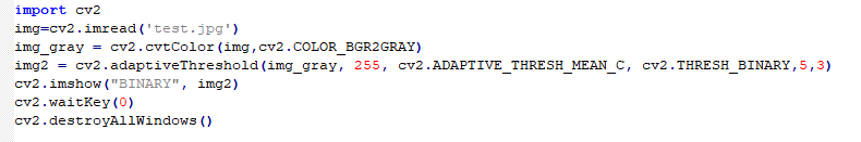
Import Module: Import cv2 module
Read Image: Call imread function to read picture and the parameter stands for the name of the picture
Color Space Conversion: call cvtColor function to convert the image into GRAY color space and the parameter indicates the picture and conversion mode.
img2 = cv2.adaptiveThreshold(img_gray, 255, cv2.ADAPTIVE_THRESH_MEAN_C, cv2.THRESH_BINARY,5,3)
Thresholding: use adaptiveThreshold function to execute. The specific format and parameters are as follow.
adaptiveThreshold(src, maxValue, adaptiveMethod, thresholdType, blockSize, C)
The first parameter
srcrefers to the pending image.The second parameter
maxValuewill be set only when the type is “cv2.THRESH_BINARY” or “cv2.THRESH_BINARY_INV”. It refers to the new value assigned when the gray values of the picture pixels are greater (smaller) than the thresholdThe third parameter
adaptiveMethoddecides how the adaptive threshold value is calculated. And the specific methods are as follow.
cv2.ADAPTIVE_THRESH_MEAN_C: set the weight value of all pixels in the neighborhood as the same.
cv2.ADAPTIVE_THRESH_GAUSSIAN_C: Obtain the weight value of all the pixels in the neighborhood through Gaussian formula. The weight value is associated with the distance between pixels in each neighbor and target pixel. The shorter the distance, the greater the weight value. The longer the distance, the smaller the weight value.
The fourth parameter
thresholdTypeindicates the type of the thresholding, which is combined with maxValue to use. This parameter only can be set as cv2.THRESH_BINARY or cv2.THRESH_BINARY_INV.The fifth parameter “blockSize” represents the size of the neighbour area. It is generally set as 3, 5, 7, ect.
The sixth parameter “C” is a constant. The threshold is mean or weight value minus this constant.
Display image: Call imshow function to display image and the parameter in bracket refers to the title of the window and displayed image.
Close window: waitKey function will wait until the keyboard is pressed, and then execute destroyAllWindows function to close the window.
Otsu Thresholding
Appropriate threshold will be automatically calculated.
1. Operation Steps
Note
Before operation, please copy the routine “Otsu_demo.py” and sample picture “test.jpg” in “6. OpenCV Computer Vision Course->6.2 Basic Course->6.2.12 Image Processing — Thresholding->Routine Code” to the shared folder.
The input command should be case sensitive and the keywords can be complemented by “Tab” key.
Open virtual machine and start the system. Click “
”, and then “” or press “Ctrl+Alt+T” to open command line terminal.Input command “cd /mnt/hgfs/share/” and press Enter to enter the shared folder.
cd /mnt/hgfs/share/
Input command “python3 Otsu_demo.py” and press Enter to run the routine.
python3 Otsu_demo.py
2. Program Outcome
The final output picture is as above.
3. Code Analysis
The Otsu thresholding, also known as the maximum inter-class variance method, is a method where the inter-class variance is calculated by assigning pixels into two or more classes. When the variance reaches the maximum value, the class dividing line i.e. the gray value is used as the image segmentation threshold.
The routine “Otsu_demo.py” can be found in “6. OpenCV Computer Vision Course->6.2 Basic Course->6.2 Basic Course->6.2.12 Image Processing—Thresholding->Routine Code”.
import cv2
img=cv2.imread('test.jpg')
img_gray = cv2.cvtColor(img,cv2.COLOR_BGR2GRAY)
ret, img2 = cv2.threshold(img_gray, 0, 255, cv2.THRESH_BINARY+cv2.THRESH_OTSU)
#the threshold is 127
#set maxval as 255. And the output image after processing is black-and-white image
cv2.imshow("BINARY", img2)
cv2.waitKey(0)
cv2.destroyAllWindows()
Otsu thresholding is to pass a parameter “cv2.THRESH_OTSU” in the parameter type of threshold function, so as to realize Otsu threshold segmentation.
In cv2.threshold(img, 0, 255, cv2.THRESH_BINARY+cv2.THRESH_OTSU),parameter thresh needs to set as 0, and parameter type should be set as “cv2.THRESH_BINARY+cv2.THRESH_OTSU”
6.2.13 Image Processing—Contour Introduction and Feature
Contour Introduction
Contour is defined as the line joining all the points along the boundary of an image that are having the same color or intensity. Contour is useful tool for shape analyzing as well as object detection and recognition.
For higher accuracy, binaryzation will be performed first. After the binary image is obtained, search the contour that is find the white object under the black background. Therefore, our target is the white object and the background is black.
Search and Draw Contour
After the object is found, search for the contour points and draw the contour.
1. Operation Steps
Note
Before operation, please copy the routine “contours_demo.py” and sample picture “test.jpg” in “6. OpenCV Computer Vision Course->6.2 Basic Course->6.2.13 Image Processing — Contour Introduction and Feature->Routine Code” to the shared folder.
The input command should be case sensitive and the keywords can be complemented by “Tab” key.
Open virtual machine and start the system. Click “
 ”, and then “
 ” or press “Ctrl+Alt+T” to open command line terminal.
Input command “cd /mnt/hgfs/share/” and press Enter to enter the shared folder.
cd /mnt/hgfs/share/
Input command “python3 contours_demo.py” and press Enter to run the routine.
python3 contours_demo.py
2. Program Outcome
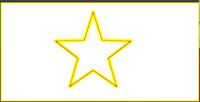
The final output picture is as above.
3. Code Analysis
The routine “contours_demo.py” can be found in “6. OpenCV Computer Vision Course->6.2 Basic Course->6.2.13 Image Processing — Contour Introduction and Feature->Routine Code”.
import cv2
img=cv2.imread('test.jpg')
img_gray = cv2.cvtColor(img,cv2.COLOR_BGR2GRAY)
ret, img2 = cv2.threshold(img_gray, 127, 255, cv2.THRESH_BINARY)
binary,contours, hierarchy = cv2.findContours(img2, cv2.RETR_TREE, cv2.CHAIN_APPROX_SIMPLE)
img3 = cv2.drawContours(img, contours, -1, (0,255,255), 3)
cv2.imshow("BINARY", img)
cv2.waitKey(0)
cv2.destroyAllWindows()
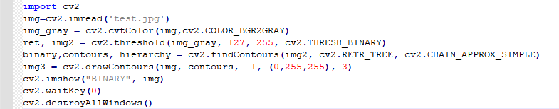
Import Module:Import cv2 module
Read Picture:Call imread function to read picture and the parameter stands for the name of the picture.
Color Space Conversion: call cvtColor function to convert the image into GRAY color space, and the parameter indicates the picture and conversion mode.
ret, img2 = cv2.threshold(img_gray, 127, 255, cv2.THRESH_BINARY)
Thresholding: use threshold function to execute. The specific format and parameters are as follow.
threshold(src, thresh, maxval, type)
The first parameter
srcis the pending image.The second parameter
threshis the set threshold.The third parameter
maxvalwill be set only when the type isTHRESH_BINARYor “THRESH_BINARY_INV”. It refers to the new value assigned when the gray values of the picture pixels are greater (smaller) than the thresholdThe fourth parameter
typerepresents the type of thresholding. cv2.THRESH_BINARY indicates the part greater than threshold is set as maxval, otherwise 0
binary,contours, hierarchy = cv2.findContours(img2, cv2.RETR_TREE, cv2.CHAIN_APPROX_SIMPLE)
Search for contour: findContours function is employed to search the contour, and the specific format and parameters are as follow.
findContours(img,mode,method)
The first parameter
imgrepresents the pending picture.The second parameter
moderepresents the detection mode of the contour.
RETR_EXTERNAL = 0: only the outermost contour will be detected
RETR_LIST = 1: detect all the contours without building hierarchy and all the contours will be put into one list
RETR_CCOMP = 2,detect all the contour and divide them into two layers
RETR_TREE = 3,Detect layer by layer from right to left according to the tree-shaped storage contour
The third parameter
methodstands for the method used to search the contour. The specific method is as follow.
CHAIN_APPROX_NONE, Preserve all the dots on the contour
CHAIN_APPROX_SIMPLE: Compress the horizontal, vertical and oblique part that is only keep their corner coordinate. For example, 4 dots are enough to save the information about the rectangle contour.
Note
In OpenCV4.2 or above, this function will only return two values, including “contours” and “hierarchy”. And “binary” will not be returned.
img3 = cv2.drawContours(img, contours, -1, (0,255,255), 3)
Contour drawing: adopt drawContours function to draw the contour, and its specific format and parameters are as follow.
drawContours(image, contours, contourIdx, color, thickness)
The first parameter
imagerepresents the image whose contour will be drawn.The second parameter
contoursrepresents the coordinate of all contours are found.The third parameter
contoursIdxindicates the serial number of the contour drawing. -1 means that all the contours will be drawn.The fourth parameter
colorrefers to the color of the contour.The fifth parameter
thicknessrepresents the width of the contour. -1 means that the contour will be padded.
Contour Feature Moment
Feature moment is global feature of a contour and a picture. The moment contains the geometric features in different types of the corresponding objects. There are three types of moments, including spatial moment, central moment and normalized central moment
Spatial moment: it is also called geometric moment about the area and perimeter of the image, including zero-order moment: m00, first-order moment: m10, m01, second-order moment: m20, m11, m02, third-order moment: m30, m21, m12, m03
Central moment: For the higher–order image, the moment will vary with the position, which can be fixed by central moment. The invariance of translation can be obtained by subtracting the mean value, so we can compare whether two objects at different positions are consistent, that is, the central moment features translation invariance.
It includes two-order central moments: mu20, mu11 and mu02, as well as three-order central moment: mu30, mu21, mu12 and mu03.
Normalized central moment: Apart from translation, some pictures will be scaled. Even though the image is scaled, its features can be detected. Normalized central moment obtain the scale invariance by dividing by the dimension of the object.
It includes two-order Hu moment: nu20, nu11 and nu02, and three-order Hu moment: nu30, nu21, nu12 and nu03. Following, based on the obtained contour, calculate the feature moment, area and perimeter of the contour.
1. Operation Steps
Note
Before operation, please copy the routine “moments_demo.py” and sample picture “test.jpg” in “6. OpenCV Computer Vision Course->6.2 Basic Course->6.2.13 Image Processing — Contour Introduction and Feature->Routine Code” to the shared folder.
The input command should be case sensitive and the keywords can be complemented by “Tab” key.
Open virtual machine and start the system. Click “
”, and then “” or press “Ctrl+Alt+T” to open command line terminal.Input command “cd /mnt/hgfs/share/” and press Enter to enter the shared folder.
cd /mnt/hgfs/share/
Input command “python3 moments_demo.py” and press Enter to run the routine.
python3 moments_demo.py
2. Program Outcome
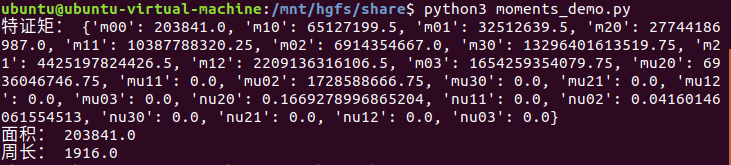
The unit of the area and perimeter is pixel. The outermost contour of the image will be calculated
3. Code Analysis
The routine “moments_demo.py” can be found in “6. OpenCV Computer Vision Course->6.2 Basic Course->6.2.13 Image Processing — Contour Introduction and Feature->Routine Code”.
import cv2
img=cv2.imread('test.jpg')
img_gray = cv2.cvtColor(img,cv2.COLOR_BGR2GRAY)
ret, img2 = cv2.threshold(img_gray, 127, 255, cv2.THRESH_BINARY)
binary,contours, hierarchy = cv2.findContours(img2, cv2.RETR_TREE, cv2.CHAIN_APPROX_SIMPLE)
cnt=contours[0]
m=cv2.moments(cnt)
area=cv2.contourArea(cnt)
perimeter=cv2.arcLength(cnt,True)
print("特证矩:",m)
print("面积:",area)
print("周长:",perimeter)
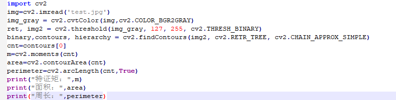
Take out the outermost contour: take the first contour with index 0 in the contour list
cnt=contours[0]
Feature moment calculation: use moments function to calculate the feature moment, and the function format and parameters are as follow.
moments(array,binaryImage)
The first parameter
arrayis the contour point.The second parameter
binaryImageis set as False by default. If it is True, all non-zero pixels will be treated as 1, which is equivalent to image binaryzation.
m=cv2.moments(cnt)
Area calculation: adopt countourArea function to calculate the area, and its format and parameters are as follow.
countourArea(contour): “contour” is a contour in the contour list.
area=cv2.contourArea(cnt)
Perimeter calculation: employ arcLength function to calculate the perimeter, and its specific format and parameter is as follow.
arcLength(curve,closed)
The first parameter
curverepresents the contour.The second parameter
closeddecide whether the contour is closed or not. If it is closed, set is asTrue, otherwise False.
perimeter=cv2.arcLength(cnt,True)
Polygon Approximation
The searched “contours” maybe too complex and not smooth, approxPolyDP function can be adopted to appropriately approximate the polygon curve, which is polygon approximation.
This function uses polygons to approximate the contour, utilizing the Douglas-Peucker algorithm (DP). The principle of the DP algorithm is simple. Its core is to continuously find the farthest point of the polygon to form a new polygon until the shortest distance is less than the specified accuracy.
Next, analyze the object contour with polygon approximation.
1. Operation Steps
Note
Before operation, please copy the routine “approx_demo.py” and sample picture “test.jpg” in “6. OpenCV Computer Vision Course->6.2 Basic Course->6.2.13 Image Processing — Contour Introduction and Feature->Routine Code” to the shared folder.
The input command should be case sensitive and the keywords can be complemented by “Tab” key.
Open virtual machine and start the system. Click “
”, and then “” or press “Ctrl+Alt+T” to open command line terminal.Input command “cd /mnt/hgfs/share/” and press Enter to enter the shared folder.
cd /mnt/hgfs/share/
Input command “python3 approx_demo.py” and press Enter to run the routine.
python3 approx_demo.py
2. Program Outcome
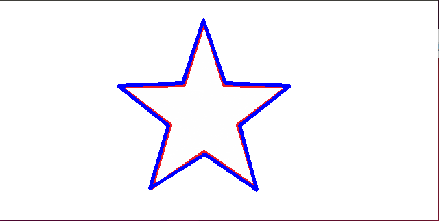
The contour after polygon approximation will try to fit the figure as much as possible.
3. Code Analysis
The routine “approx_demo.py” can be found in “6. OpenCV Computer Vision Course->6.2 Basic Course->6.2.13 Image Processing—Contour Introduction and Feature->Routine Code”.
import cv2
img=cv2.imread('test.jpg')
img_gray = cv2.cvtColor(img,cv2.COLOR_BGR2GRAY)
ret, img2 = cv2.threshold(img_gray, 127, 255, cv2.THRESH_BINARY)
binary,contours, hierarchy = cv2.findContours(img2, cv2.RETR_TREE, cv2.CHAIN_APPROX_SIMPLE)
cnt=contours[1]
approxl=cv2.approxPolyDP(cnt,20,True)
img3 = cv2.drawContours(img, [approxl], -1, (255,0,0), 3)
cv2.imshow("BINARY", img)
cv2.waitKey(0)
cv2.destroyAllWindows()
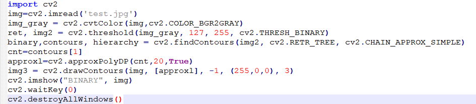
Take the contour: take the second contour with index 1 in the contour list
cnt=contours[1]
Polygon approximation: apporxPolyDP function is adopted. The specific format is as follow.
apporxPolyDP(curve, epsilon, closed)
The first parameter
curveis the contour to be searched.The second parameter
epsilonindicates accuracy. The smaller the number, the lower the accuracy and the more consistent with the pattern contour.The third parameter
closeddecide whether the contour is closed or not. If it is closed, set is asTrue, otherwise False.
approxl=cv2.approxPolyDP(cnt,20,True)
Contour Convex Hull
Convex Hull will look similar to contour approximation, but it is the convex polygon in the outermost of the object. Convex hull refers to a polygon that completely contains the original contour and consists only of points on the contour. Every part of the convex hull is convex, that is, the line connecting any two points in the convex hull is inside the convex hull. In the convex hull, the interior angle of any three consecutive points is less than 180°.
Next, analyze the object contour through contour convex hull.
1. Operation Steps
Note
Before operation, please copy the routine “hull_demo.py” and sample picture “test.jpg” in “6. OpenCV Computer Vision Course->6.2 Basic Course->6.2.13 Image Processing — Contour Introduction and Feature->Routine Code” to the shared folder.
The input command should be case sensitive and the keywords can be complemented by “Tab” key.
Open virtual machine and start the system. Click “
”, and then “” or press “Ctrl+Alt+T” to open command line terminal.Input command “cd /mnt/hgfs/share/” and press Enter to enter the shared folder.
cd /mnt/hgfs/share/
Input command “python3 hull_demo.py” and press Enter to run the routine.
python3 hull_demo.py
2. Program Outcome
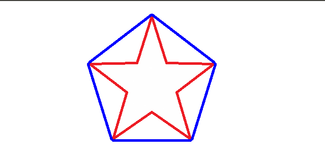
The convex hull will connect the vertices of the contour.
3. Code Analysis
The routine “hull_demo.py” can be found in “6. OpenCV Computer Vision Course->6.2 Basic Course->6.2.13 Image Processing—Contour Introduction and Feature->Routine Code”
import cv2
img=cv2.imread('test.jpg')
img_gray = cv2.cvtColor(img,cv2.COLOR_BGR2GRAY)
ret, img2 = cv2.threshold(img_gray, 127, 255, cv2.THRESH_BINARY)
binary,contours, hierarchy = cv2.findContours(img2, cv2.RETR_TREE, cv2.CHAIN_APPROX_SIMPLE)
cnt=contours[1]
hull=cv2.convexHull(cnt,True)
img3 = cv2.drawContours(img, [hull], -1, (255,0,0), 3)
cv2.imshow("BINARY", img)
cv2.waitKey(0)
cv2.destroyAllWindows()
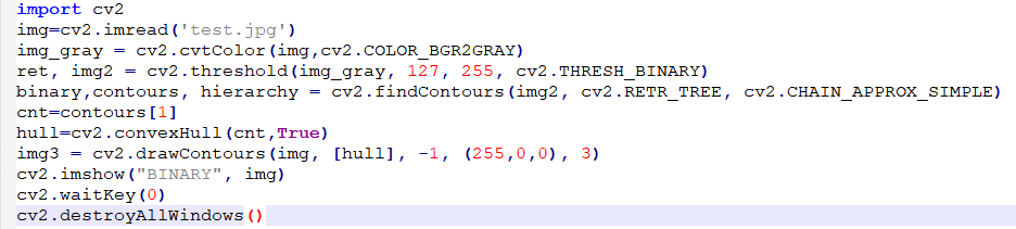
Convex hull: use convexHull function to draw the convex hull. The function format and parameters are as follow.
convexHull(points, clockwise,)
The first parameter
pointsis the contour to be searched.The second parameter
clockwiserefers to the drawing direction. When it is True, the convex hull will be draw clockwise. When it is False, the convex hull will be drawn counterclockwise.
hull=cv2.convexHull(cnt,True)
Circumscribed Rectangle
The bounding rectangle is divided into the minimum bounding rectangle with rotation angle and the regular circumscribed rectangle.
Minimum bounding rectangle: it is drawn with minimum area, so it considers the rotation.
Regular bounding rectangle: frame the object with the rectangle.
Next, draw the regular bounding rectangle and minimum bounding rectangle.
1. Operation Steps
Note
Before operation, please copy the routine “rect_demo.py” and sample picture “test.jpg” in “6. OpenCV Computer Vision Course->6.2 Basic Course->6.2.13 Image Processing — Contour Introduction and Feature->Routine Code” to the shared folder.
The input command should be case sensitive and the keywords can be complemented by “Tab” key.
Open virtual machine and start the system. Click “
”, and then “” or press “Ctrl+Alt+T” to open command line terminal.Input command “cd /mnt/hgfs/share/” and press Enter to enter the shared folder.
cd /mnt/hgfs/share/
Input command “python3 rect_demo.py” and press Enter to run the routine.
python3 rect_demo.py
2. Program Outcome
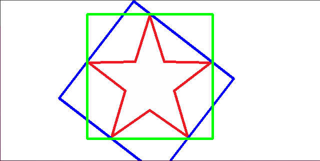
The green one is the regular bounding rectangle, and the blue one is the minimum bounding rectangle.
3. Code Analysis
The routine “rect_demo.py” can be found in “6. OpenCV Computer Vision Course->6.2 Basic Course->6.2.13 Image Processing—Contour Introduction and Feature->Routine Code”
import cv2
import numpy as np
img=cv2.imread('test.jpg')
img_gray = cv2.cvtColor(img,cv2.COLOR_BGR2GRAY)
ret, img2 = cv2.threshold(img_gray, 127, 255, cv2.THRESH_BINARY)
binary,contours, hierarchy = cv2.findContours(img2, cv2.RETR_TREE, cv2.CHAIN_APPROX_SIMPLE)
cnt=contours[1]
RotatedRect=cv2.minAreaRect(cnt)
x,y,w,h=cv2.boundingRect(cnt)
box=cv2.boxPoints(RotatedRect)
box=np.int0(box)
img3 = cv2.drawContours(img, [box], -1, (255,0,0), 3)
img4=cv2.rectangle(img,(x,y),(x+w,y+h),(0,255,0),3)
cv2.imshow("BINARY", img)
cv2.waitKey(0)
cv2.destroyAllWindows()
Acquire minimum bounding rectangle: adopt minAreaRect function to get the minimum bounding rectangle. And the function format and parameters are as follow.
minAreaRect( points ): “points” refers to contour, and the returned value contains the starting coordinate, width, height and angle.
RotatedRect=cv2.minAreaRect(cnt)
Obtain the regular bounding rectangle: use “boundingRect” function to realize. The function format and parameters are as follow.
boundingRect(array): “array” refers to contour and the returned value “Rect” contains the starting coordinate, width and height.
x,y,w,h=cv2.boundingRect(cnt)
Get the vertex coordinate of the minimum bounding rectangle: boxPoints function will be employed. The function format and parameters are as follow.
boxPoints(rect): refers to the rectangle whose vertex coordinate needs to be obtained. Its data type belongs to floating point number.
box=cv2.boxPoints(RotatedRect)
Number rounding: use int0 function to execute. The function format and parameters are as follow.
int0(date): “date” is the data to be rounded.
box=np.int0(box)
Draw rectangle: rectangle function will be adopted to draw the rectangle. The function format and parameters are as follow.
rectangle(src,pt1,pt2,color,thickness)
The first parameter
srcrefers to the image to draw the contour.The second parameter
pt1represents one of the vertices of the rectangle.The third parameter
pt2refers to the diagonal vertices of pt1The fourth parameter
colorrepresents the color of the rectangle.The fifth parameter
thicknessrepresents the width of the drawn rectangle. “-1” indicates padding rectangle.
img4=cv2.rectangle(img,(x,y),(x+w,y+h),(0,255,0),3)
6.2.14 Image Processing—Feature Matching
Brute-Force Matching
The feature descriptor is to describe the key point with a set of vectors after the key point is calculated. It includes not only the key point, but also the pixels around the key point that has made a contribution. It serves as the basis for target matching, and enables the key points to have more invariant characteristics, such as illumination changes, 3D viewpoint changes, etc.
Each feature descriptor in one set of features is matched with the nearest feature descriptor of the other set, then the obtained distances are sorted, and finally the feature with the shortest distance is selected as the matching point for the two.
Next, use brute force matching to match the features of the two images.
1. Operation Steps
Note
Before operation, please copy the routine “bf_demo.py” and sample picture “test.jpg” in “6. OpenCV Computer Vision Course->6.2 Basic Course->6.2.14 Image Processing — Feature Matching->Routine Code” to the shared folder.
The input command should be case sensitive and the keywords can be complemented by “Tab” key.
Open virtual machine and start the system. Click “
 ”, and then “
 ” or press “Ctrl+Alt+T” to open command line terminal.
Input command “cd /mnt/hgfs/share/” and press Enter to enter the shared folder.
cd /mnt/hgfs/share/
Input command “python3 bf_demo.py” and press Enter to run the routine.
python3 bf_demo.py
2. Program Outcome
Take out one part of the original image, and then match features between these two images.
3. Code Analysis
The routine “bf_demo.py” can be found in “6. OpenCV Computer Vision Course->6.2 Basic Course->6.2.14 Image Processing — Feature Matching->Routine Code”.
import cv2

img1 = cv2.imread('test.jpg')
img2=cv2.imread('test1.jpg')

# initialize ORB feature detector
orb = cv2.ORB_create()

# detect feature and descriptor
kp1, des1 = orb.detectAndCompute(img1,None)
kp2, des2 = orb.detectAndCompute(img2,None)

# Create a brute force (BF) matcher
bf = cv2.BFMatcher_create(cv2.NORM_HAMMING, crossCheck=True)

# match descriptor
matches = bf.match(des1,des2)

# draw ten matched descriptors
img3 = cv2.drawMatches(img1, kp1, img2, kp2, matches[:10], None, flags=2)

cv2.imshow("show",img3)
cv2.waitKey()
cv2.destroyAllWindows()
Import Module:Import cv2 module
Read Picture:Call imread function to read picture and the parameter stands for the name of the picture.
Initialized detector: use ORB_create constructor for initialization.
# initialize ORB feature detector
orb = cv2.ORB_create()
Detect feature and descriptor: detectAndCompute function will be used to detect. And the specific format and parameter are as follow.
detectAndCompute(src,mask)
The first parameter
srcis the image to process the threshold.The second parameter
maskis the image in which the object is black and the rest is white. If the mask is not required, set the parameter as None.
kp1, des1 = orb.detectAndCompute(img1,None)
kp2, des2 = orb.detectAndCompute(img2,None)
Create BFMatcher object: BFMatcher belongs to features2d module and inherits from DescriptorMatcher. The function format is as follow.
static Ptr<BFMatcher> create( int normType , bool crossCheck )
The first parameter “normType” can be set as NORM_L1, NORM_L2, NORM_HAMMING or NORM_HAMMING2. The HOG descriptors of SIFT and SURF correspond to the Euclidean distances L1 and L2; the BRIEF descriptors of ORB and BRISK correspond to the Hamming distance HAMMING; HAMMING2 corresponds to the ORB algorithm when WTA_K = 3 or 4.
Euclidean distance: it is defined as the distance between two points in n-dimensional space.
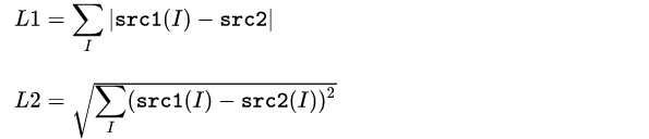
Hamming distance: It is computer’s XOR operation suitable for binary string descriptors, such as BRIEF descriptors. Its definition is as follow.
The second parameter
crossCheckis set asFALSEby default. If set as TRUE, the matching is valid only when the features in the two groups match with each other. In other words, only when the x point descriptor in group A and the y point in group B are the best matching points for each other, the matching is effective.
bf = cv2.BFMatcher_create(cv2.NORM_HAMMING, crossCheck=True)
Match descriptor: detectAndCompute function will be adopted, and its specific format and parameters are as follow. match(queryDescriptors,trainDescriptors)
The first parameter “queryDescriptors” is the image feature vector to be matched.
The second parameter “trainDescriptors” is the image feature vector that needs to be matched.
matches = bf.match(des1,des2)
Draw matches: drawMatches function will used. The specific format and parameters are as follow.
drawMatches(src1,kp1,src2,kp2,match,matchesMask,flags)
The first parameter
src1is the matching image 1.The second parameter
kp1is the feature of image 1.The third parameter
src2is the matching image 2.The fourth parameter
kp2is the feature of the image 2.The fifth parameter
matchis the set of matching points to be drawn.The sixth parameter
matchesMaskdetermines which images to draw. If it is set as None, all the images will be drawn.The seventh parameter
flagsrepresents the drawing flag. 0 indicates that all the features will be drawn, and 2 indicates that only the matched feature will be drawn. 4 stands for the drawing styles.
img3 = cv2.drawMatches(img1, kp1, img2, kp2, matches[:10], None, flags=2)
Display image:Call imshow function to display image and the parameter in bracket refers to the title of the window and displayed image.
Close window: waitKey function will wait until the keyboard is pressed, and then execute destroyAllWindows function to close the window.
cv2.imshow("show",img3)
cv2.waitKey()
cv2.destroyAllWindows()
Nearest Neighbor Matching
FLANN (Fast Library for Approximate Nearest Neighbors) is a FLANN is a open-source library for performing fast approximate nearest neighbor searches in high dimensional spaces.
The nearest neighbor matching operator FlannBasedMatcher based on the FLANN library is much more efficient than BFMatcher in the field of large feature datasets or some real-time processing.
Next, adopt nearest neighbor matching to match the features of the two images.
1. Operation Steps
Note
Before operation, please copy the routine “flann_demo.py” and sample pictures “test.jpg” and “test1.jpg” in “6. OpenCV Computer Vision Course->6.2 Basic Course->6.2.14 Image Processing — Feature Matching->Routine Code” to the shared folder.
The input command should be case sensitive and the keywords can be complemented by “Tab” key.
Open virtual machine and start the system. Click “
”, and then “” or press “Ctrl+Alt+T” to open command line terminal.Input command “cd /mnt/hgfs/share/” and press Enter to enter the shared folder.
cd /mnt/hgfs/share/
Input command “python3 flann_demo.py” and press Enter to run the routine.
python3 flann_demo.py
2. Program Outcome
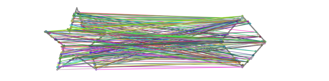
3. Code Analysis
The routine “flann_demo.py” can be found in “6. OpenCV Computer Vision Course->6.2 Basic Course->6.2.14 Image Processing—Feature Matching->Routine Code”.
import numpy as np
import cv2 as cv

img1 = cv.imread('test.jpg',cv.IMREAD_GRAYSCALE)    # index image
img2 = cv.imread('test1.jpg',cv.IMREAD_GRAYSCALE)    # training image

# initialize ORB descriptor
orb = cv.ORB_create()

# search keypoint and descriptor based on ORB
kp1, des1 = orb.detectAndCompute(img1,None)
kp2, des2 = orb.detectAndCompute(img2,None)

# parameters of FLANN
FLANN_INDEX_LSH = 6
index_params= dict(algorithm = FLANN_INDEX_LSH,
                   table_number = 6, # 12
                   key_size = 12,     # 20
                   multi_probe_level = 1) #2
search_params = dict(checks=50)   # transfer a empty dictionary
flann = cv.FlannBasedMatcher(index_params,search_params)

matches = flann.knnMatch(des1,des2,k=2)

img3 = cv.drawMatchesKnn(img1,kp1,img2,kp2,matches,None)
cv.imshow("show",img3)
cv.waitKey()
cv.destroyAllWindows()
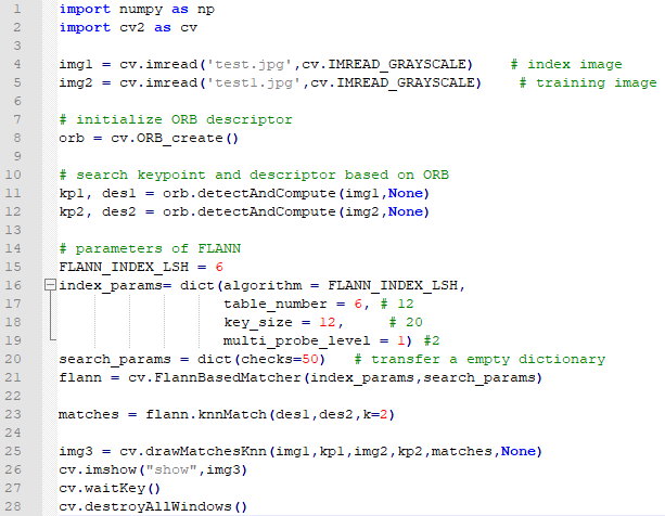
Set FLANN parameter: FlannBasedMatcher function will be adopted. And its format and parameters are as follow.
FlannBasedMatcher(IndexParams,SearchParams)(The two parameters in the bracket refers to the type of the dictionary)
The first parameter “IndexParams” the algorithm designated to use.
The second parameter “SearchParams” is the number of times the tree in the specified index should be traversed recursively. Higher values provide better accuracy, but also take more time.
index_params= dict(algorithm = FLANN_INDEX_LSH,
                   table_number = 6, # 12
                   key_size = 12,     # 20
                   multi_probe_level = 1) #2
search_params = dict(checks=50)   # transfer a empty dictionary
flann = cv.FlannBasedMatcher(index_params,search_params)
Nearest neighbor matching: knnMathch function will be used, And the function format and parameters are as follow.
knnMathch(queryDescriptors,trainDescriptors,k)
The first two parameters are consistent with match, and “k” is the best number of matches to be returned.)
matches = flann.knnMatch(des1,des2,k=2)
6.2.15 Image Processing—Corner Detection
Corner Introduction
1. Corner Definition
The corner is defined as the intersection of two edges, or a feature with two main directions in the neighborhood. In general, corner is the point on the edge curve with maximum curvature, or the point with large variation in intensity in the image.
2. Detection Idea
Define a tiny local window in the image, then move this window in all directions, which will leads to three results, including flat areas, edges and corners.
If the image intensity of window doesn’t change as the window is moving in all directions, inside the window are all flat areas, and corner isn’t involved.
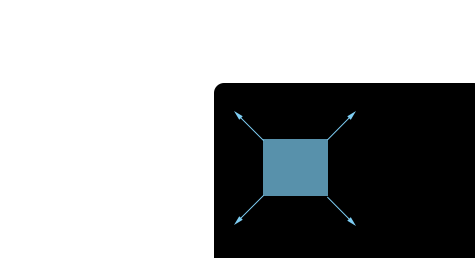
If the image intensity of window change greatly as the window is moving in one (some) direction(s), but keeps still in other directions, there maybe “edges” inside the window.
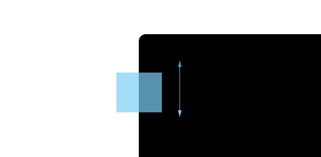
f the image intensity of window change greatly in all direction, there maybe “corners” inside the window.
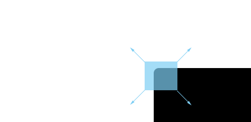
3. Harris Corner Detection Formula
And:
det(M)=λ1λ2。
trace(M)=λ1+λ2。
λ1 and λ2 are the feature values of the moment M.
The region type can be judged based on these features:
When |R| is small, which happens when λ1 and λ2 are small, the region is flat.
When R<0, which happens when λ1>>λ2 or vice versa, the region is edge.
When R is large, which happens when λ1 and λ2 are large and λ1∼λ2, the region is a corner.
Operation Steps
Next, detect the corners of the image through Harris corner detection.
Note
Before operation, please copy the routine “corners_demo.py” and sample pictures “test.jpg” in “6. OpenCV Computer Vision Course->6.2 Basic Course->6.2.15 Image Processing — Corner Detection->Routine Code” to the shared folder.
The input command should be case sensitive and the keywords can be complemented by “Tab” key.
Open virtual machine and start the system. Click “
 ”, and then “
 ” or press “Ctrl+Alt+T” to open command line terminal.
Input command “cd /mnt/hgfs/share/” and press Enter to enter the shared folder.
cd /mnt/hgfs/share/
Input command “python3 bf_demo.py” and press Enter to run the routine.
python3 bf_demo.py

Program Outcome
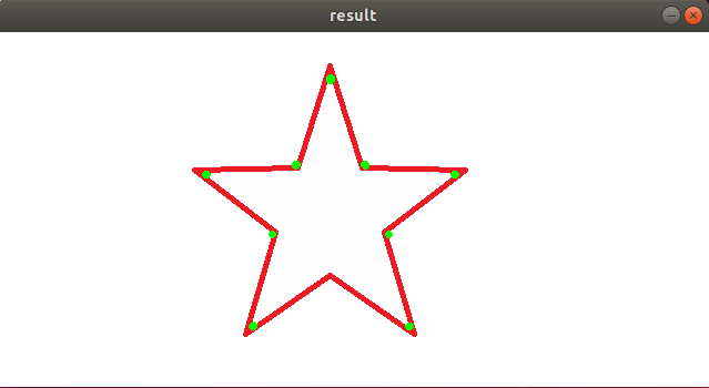
Code Analysis
The routine “corners_demo.py” can be found in “6. OpenCV Computer Vision Course->6.2 Basic Course->6.2.15 Image Processing — Corner Detection->Routine Code”
import numpy as np
import cv2 as cv


def harris(image):
    # Detector parameters
    blockSize = 2
    apertureSize = 3
    k = 0.04
    # Detecting corners
    gray = cv.cvtColor(image, cv.COLOR_BGR2GRAY)
    dst = cv.cornerHarris(gray, blockSize, apertureSize, k)
    # Normalizing
    print(dst)
    dst_norm = np.empty(dst.shape, dtype=np.float32)
    cv.normalize(dst, dst_norm, alpha=0, beta=255, norm_type=cv.NORM_MINMAX)
    # Drawing a circle around corners
    for i in range(dst_norm.shape[0]):
        for j in range(dst_norm.shape[1]):
            if int(dst_norm[i, j]) > 120:
                cv.circle(image, (j, i), 2, (0, 255, 0), 2)
    # output
    return image


src = cv.imread("test.jpg")
result = harris(src)
cv.imshow('result', result)
cv.waitKey(0)
cv.destroyAllWindows()
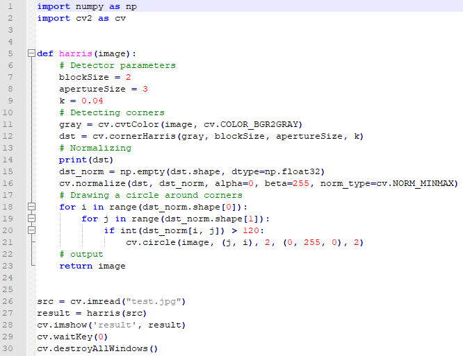
Import Module: Import cv2 and nmupy module.
gray = cv.cvtColor(image, cv.COLOR_BGR2GRAY)
Create corner detection function:harris(image):the parameter in the bracket is the image that needs to process
color space conversion:cvtColor(src,mode)
The first parameter src refers to the image to convert.
The second parameter mode is the conversion mode of the color space.
dst = cv.cornerHarris(gray, blockSize, apertureSize, k)
Corner Detection:cornerHarris(src,blockSize,apertureSize,k)
The first parameter src is the image for detection.
The second parameter blockSize is the size of the domain pixel.
The third parameter apertureSize is the size of the used window.
The fourth parameter k is a free parameter ranging [0.04,0.06].
dst_norm = np.empty(dst.shape, dtype=np.float32)
Acquire the array of the same type:empty(shape,dtype)
The first parameter shape represents the shape of the returned array defined by the integer or a tuple of integers.
The second parameter dtype refers to the data type defining the type of the returned array.
cv.normalize(dst, dst_norm, alpha=0, beta=255, norm_type=cv.NORM_MINMAX)
Normalization: Normalization is to process the data and then limit within the required range. The size of the output image of Harris corner detection after normalization is the same as the original image. Pixel value of each point corresponds to the probability that the point is corner. The greater the value, the more likely it is a corner.
Function format: normalize(src,dst,alpha,beta,normType)
The first parameter src is the input array.
The second parameter dst is the output array after processing.
The third parameter alpha is the minimum value of normalization
The fourth parameter beta is the maximum value of normalization
The fifth parameter normType indicates the types of normalization as below.
(1) NORM_MINMAX: The value of the array is translated or scaled to a specified range. Linearly normalized is commonly used.
(2) NORM_INF: it is the C-norm of the normalized array (the maximum value of the absolute value)
(3) NORM_L1: L1-norm of the normalized array (sum of absolute values)
(4) NORM_L2: (Euclidean) L2-norm of the normalized array
for i in range(dst_norm.shape[0]):
        for j in range(dst_norm.shape[1]):
            if int(dst_norm[i, j]) > 120:
                cv.circle(image, (j, i), 2, (0, 255, 0), 2)
**Circle the corner:**use a loop to traverse the normalized image array and draw a circle in the corner area.
Function format**:**circle(src,point,radius,color,thickness)
The first parameter src is the image to be drawn.
The second parameter point is the center of the drawn circle
The third parameter radius refers to the radius of the circle
The fourth parameter color is the set color
The fifth parameter thickness refers to the line thickness of the circle. When it is negative number, it is solid circle.
src = cv.imread("test.jpg")
result = harris(src)
cv.imshow('result', result)
cv.waitKey(0)
cv.destroyAllWindows()
Read image, process image, display image and close the window:
Read image: Use imread(image) function to read the image, and the parameter in the bracket is the name of the picture
Process image: call harris(image) function to process the image and the image parameters will be passed in.
Display image: employ imshow(title,src) function to display the output image. The parameters in the bracket are the title of window and the displayed image.
Close window:Adopt waitKey function to wait for the key to be pressed, and then call destroyAllWindows function to close the display window.