2. Chassis Motion Control Course
2.1 Motion Control
2.1.1 IMU Calibration
Note
The robot is factory-calibrated and generally does not require recalibration. This section is provided for reference only. If the robot deviates significantly during navigation—for example, drifting noticeably to one side while moving forward and unable to drive in a straight line, follow the tutorial below to perform calibration.
Calibration is intended to reduce errors. Some hardware deviations are inevitable, so the goal is to adjust the settings to achieve a performance that is relatively accurate and meets your needs.
If deviations occur during use, the IMU, linear velocity, and angular velocity should be recalibrated. After calibration, the robot can perform all its functions correctly.
The IMU, Inertial Measurement Unit, is a device that measures an object’s three-axis orientation, angular velocity, and acceleration. The gyroscope and accelerometer are the main components of the IMU, providing a total of six degrees of freedom to measure angular velocity and acceleration in 3D space.
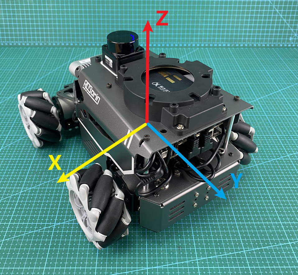
The figure above shows the positive directions of the IMU’s x, y, and z axes. During the calibration process, you can refer to this coordinate system. After the node receives the first IMU message, it will prompt you to hold the IMU in a specific orientation and press Enter to record the measurement. Once all six orientations are completed, the node calculates the calibration parameters and writes them to the specified YAML file. The detailed steps are as follows:
Note
The input command should be case sensitive, and the keywords can be complemented by the Tab key.
Power on the robot and connect it via the NoMachine remote control software. For detailed information, please refer to the section 1.7 Development Environment Setup in the user manual.
Click the terminal icon
 in the system desktop to open a command-line window.
Enter the following command and press Enter to stop the app auto-start service.
sudo systemctl stop start_app_node.service
Next, enter the command and press Enter to start the chassis control node:
ros2 launch ros_robot_controller ros_robot_controller.launch.py
Then, open a new terminal, enter the command, and press Enter to start the IMU calibration:
ros2 run imu_calib do_calib --ros-args -r imu:=/ros_robot_controller/imu_raw --param output_file:=/home/ubuntu/ros2_ws/src/calibration/config/imu_calib.yaml
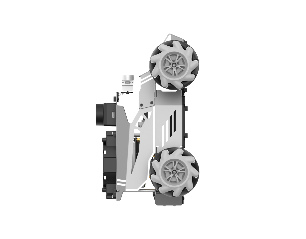
When the command line terminal displays the following prompt, it indicates that calibration of the IMU’s X-axis angular velocity offset in the positive direction is ready to start. Next, tilt the robot to the side so that the orientation matches the figure below, ensuring both the direction and angle are correct. Then, press Enter to execute.

After each orientation is successfully calibrated, the following prompts will appear:

When the command line terminal displays the following prompt, it indicates that calibration of the IMU’s X-axis angular velocity offset in the negative direction is ready to start. Next, tilt the robot to the side so that the orientation matches the figure below, ensuring both the direction and angle are correct. Then, press Enter to execute.

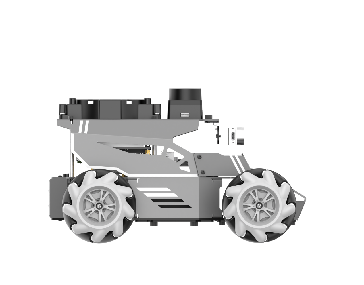
Next, when the command line terminal displays the following prompt, it indicates that calibration of the IMU’s Y-axis angular velocity offset in the positive direction is ready to start. Place the robot upright according to the orientation shown in the figure below, ensuring the direction and angle match the diagram. Then, press Enter to execute.

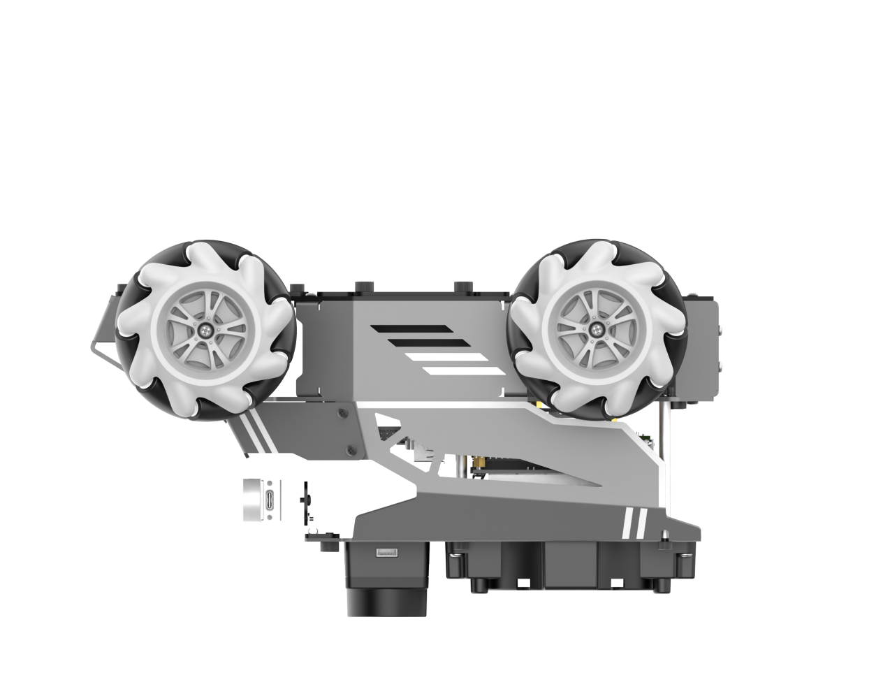
When the command line terminal shows the next prompt, it indicates that calibration of the IMU’s Y-axis angular velocity offset in the negative direction is ready to start. Position the robot face-down following the orientation shown in the diagram, making sure its direction and angle match the reference. Then, press Enter to proceed.

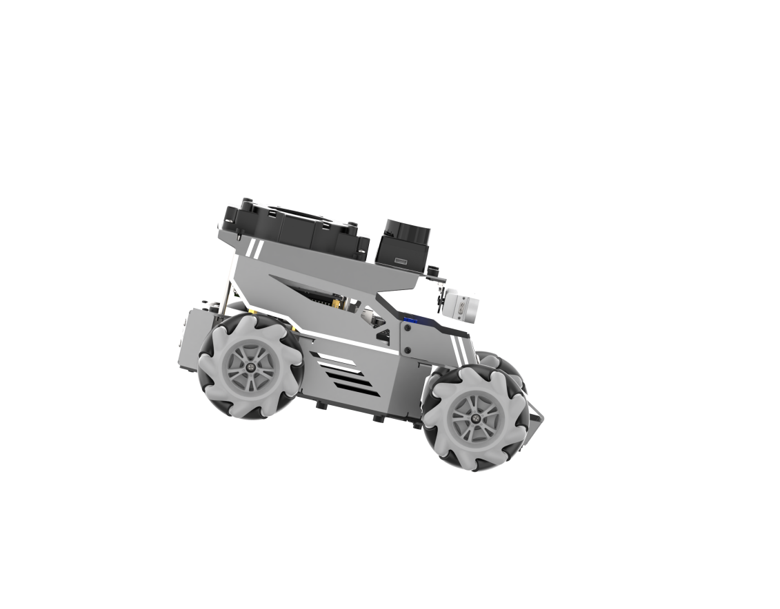
When the command line terminal displays the next prompt, it indicates that calibration of the IMU’s Z-axis angular velocity offset in the positive direction is ready to start. Pick up the robot, hold it upright facing upward, keep it steady, and press Enter to continue. Hold the robot in the orientation shown in the image, making sure the direction and angle match the diagram, then press Enter to proceed.

The terminal will then display a prompt indicating that the negative Z-axis gyroscope offset can be calibrated. Position the robot as shown in the diagram, ensuring its orientation and angle match the reference, and press Enter to continue.

When the following message appears, the calibration is complete. Press Ctrl+C to exit.

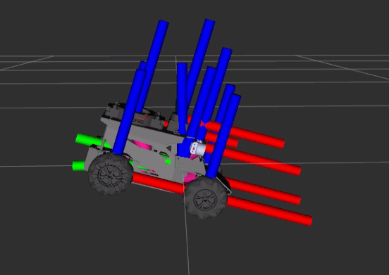
After calibration, you can check the calibrated model by running the command:
ros2 launch peripherals imu_view.launch.py
Gently tilt the platform to check whether the model’s tilt direction matches the actual movement. Refer to the example below. If both directions align, the IMU calibration results are considered accurate.
2.1.2 Angular Velocity Calibration
When the robot shows noticeable deviation in turning points or turning angles during mapping, navigation, or routine driving, angular-velocity calibration is required. The process is as follows:
Note
Commands must be entered with correct capitalization. The Tab key can be used to auto-complete keywords.
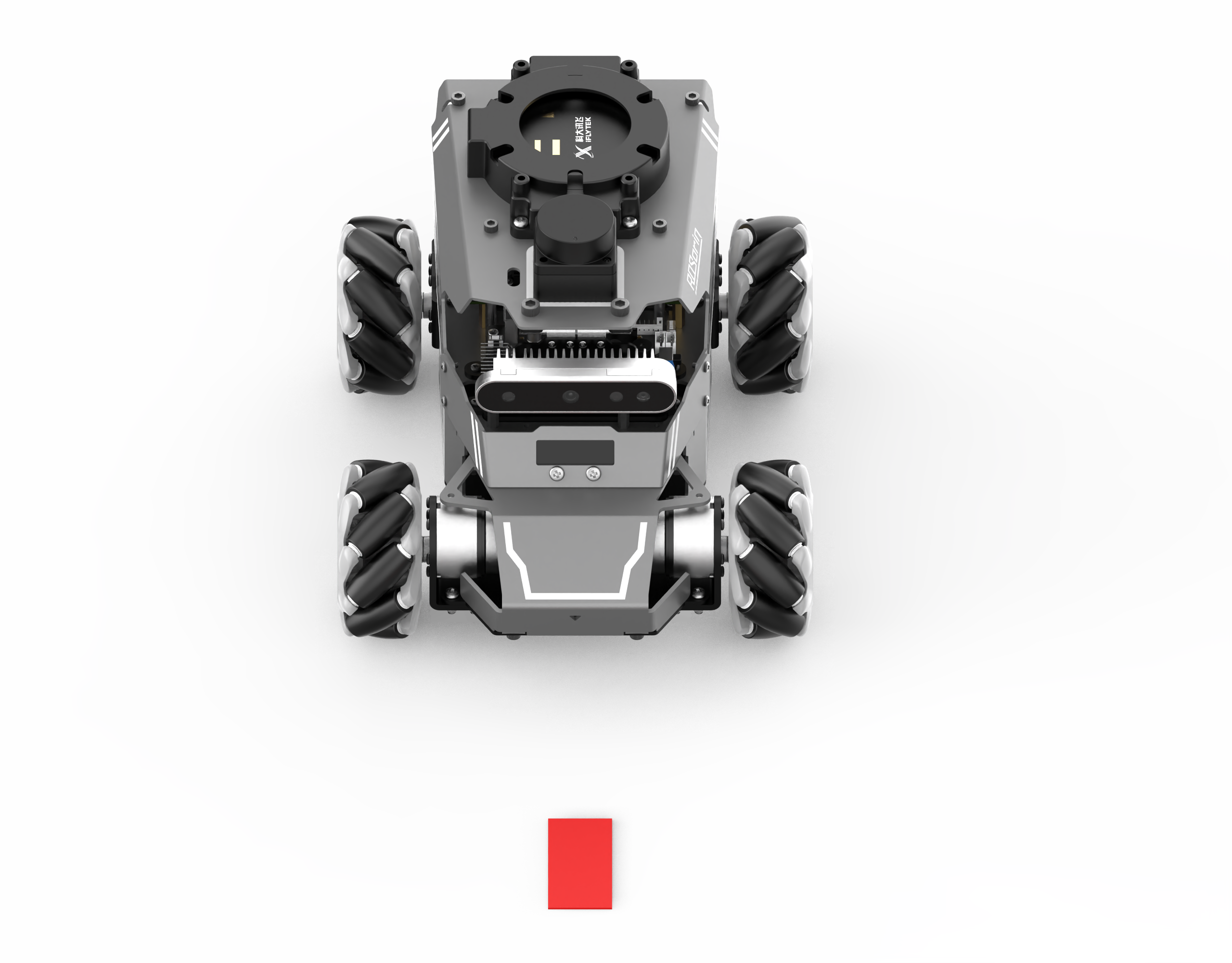
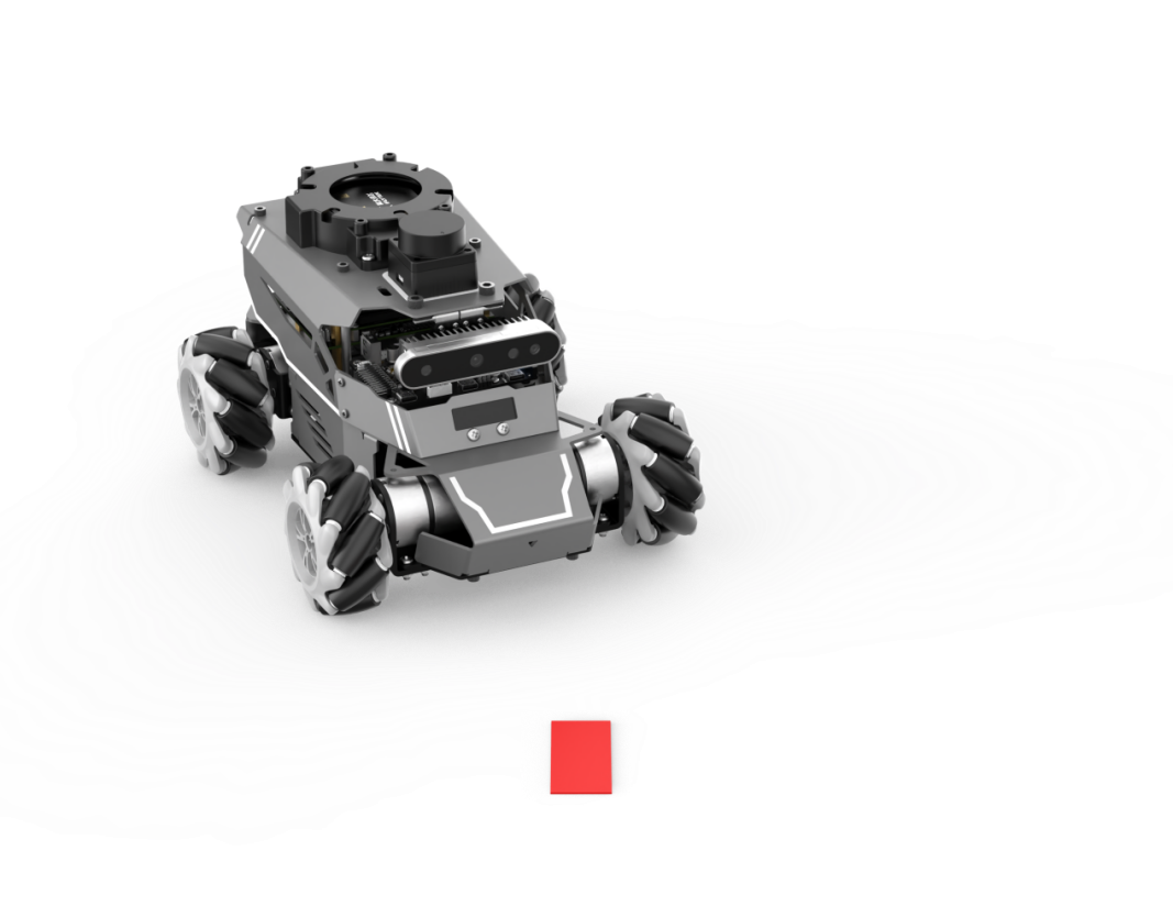
Place the robot on a flat surface and apply a piece of tape—or position another marker—at the center of its front side, as shown below.
Power on the robot and connect to it using the remote connection tool by following the section 1.7.2 AP Mode Connection Steps in the user manual.
Click the terminal icon
on the system desktop.Enter the following command and press Enter to stop the app auto-start service.
sudo systemctl stop start_app_node.service
Before starting the calibration, navigate to the calibration configuration file directory and open the configuration file.
cd ~/ros2_ws/src/driver/controller/config && vim calibrate_params.yaml
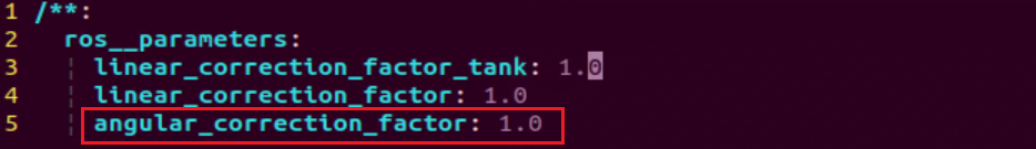
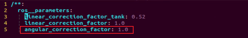
Set the angular velocity parameter to 1.0 before proceeding with the calibration.
After editing, press ESC, type
:wq, and press Enter to save and exit.Next, enter the command and press Enter to start the chassis control node:
ros2 launch ros_robot_controller ros_robot_controller.launch.py
Then, open a new terminal, enter the command, and press Enter to start the angular velocity calibration:
ros2 launch calibration angular_calib.launch.py
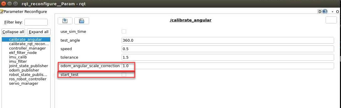
Then, click calibrate_angular on the left to open the calibration interface, as shown below.
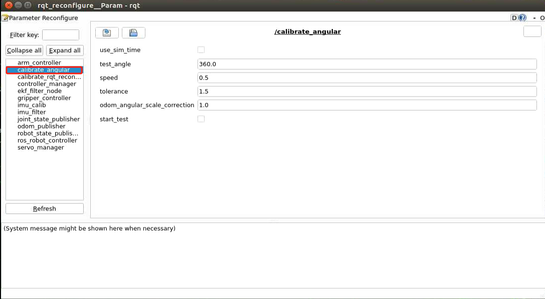
The meanings of the parameters on the left side of the interface are as follows:
(1) test_angle – The rotation angle for testing, 360° by default.
(2) speed – The linear speed, default is 0.15 m/s.
(3) tolerance – The allowable error. A smaller error value results in more noticeable oscillation when the robot reaches its target position.
(4) odom_angule_scale_correction – The odometry angle scaling ratio.
(5) start_test – Button to start testing the odometry angle scaling.
Make sure the robot is properly aligned, then check start_test. The robot will rotate in place. If it cannot complete a full rotation or shows deviation, adjust the odom_angle_scale_correction value, which scales the motor rotation during turning. It is recommended to adjust in increments of 0.01 and repeat the test until the robot can rotate exactly one full turn, then record this value.
If the rotation angle exceeds one full turn, it indicates a deviation in the robot’s angular velocity. To correct it, increase the odom_angular_scale_correction parameter in the input field next to the slider, adjusting by 0.01 each time. For example, changing 1.0 to 1.01. Conversely,
If the rotation angle is less than one full turn, decrease the parameter odom_angular_scale_correction.
When the robot completes exactly one full turn, the calibration is correct. Record the current value of odom_angular_scale_correction.
After calibration, open the calibration configuration file to save the corrected parameter:
cd ~/ros2_ws/src/driver/controller/config && vim calibrate_params.yaml
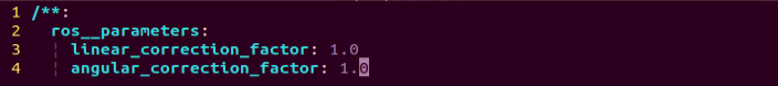
Press the key i to enter edit mode and modify the value of angular_correctqion_factor to the calibrated value of odom_angule_scale_correction.
Note
This section uses the Mecanum chassis as an example for calibration. The Ackermann chassis does not require angular velocity calibration.
After editing, press ESC, type
:wq, and press Enter to save and exit.
2.1.3 Linear Velocity Calibration
Note
Commands must be entered with correct capitalization. The Tab key can be used to auto-complete keywords.
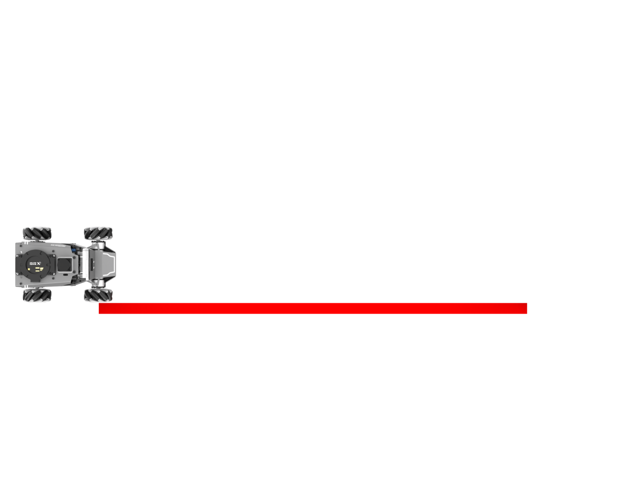
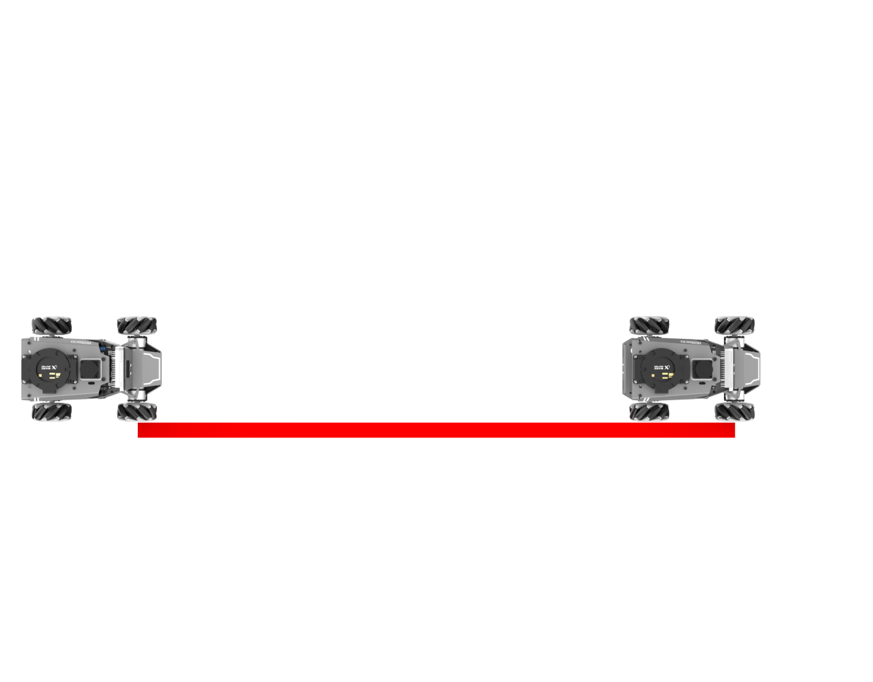
Place the robot on a flat, open surface. Attach a start marker, such as tape, directly in front of the platform, and place an end marker about 1 meter ahead, as shown below.
Power on the robot and connect to it using the remote connection tool by following the section 1.7.2 AP Mode Connection Steps in the user manual.
Click the terminal icon
in the system desktop to open a command-line window.Enter the following command and press Enter to stop the app auto-start service.
sudo systemctl stop start_app_node.service
Before starting the calibration, navigate to the calibration configuration file directory and open the configuration file.
cd ~/ros2_ws/src/driver/controller/config && vim calibrate_params.yaml
Change the linear velocity parameter linear_correction_factor to 1.0 before proceeding with the calibration.
After editing, press ESC, type
:wq, and press Enter to save and exit.Next, enter the command and press Enter to start the chassis control node:
ros2 launch ros_robot_controller ros_robot_controller.launch.py
Then, open a new terminal, enter the command, and start the linear velocity calibration:
ros2 launch calibration linear_calib.launch.py
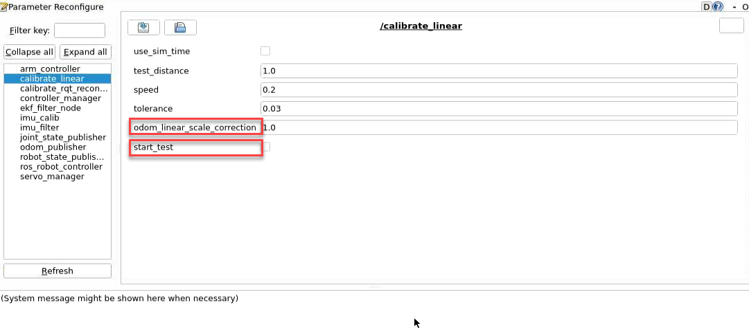
After the calibration program starts, click on calibrate_linear on the left to open the calibration interface, as shown below:
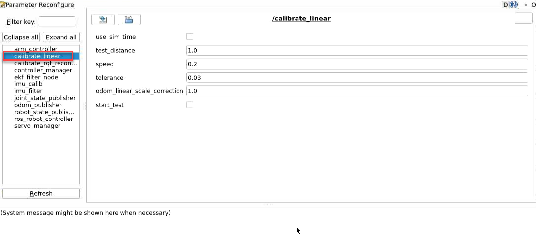
The meanings of the parameters on the left side of the interface are as follows:
(1) test_distance – The test distance, default is 1 meter.
(2) speed – The linear speed, default is 0.2 m/s.
(3) tolerance – The allowable error. Smaller values reduce the deviation from the target but may cause more shaking after reaching the target.
(4) odom_linear_scale_correction – The odometry linear scale factor.
(5) start_test – The button to start testing the odometry linear scale factor.
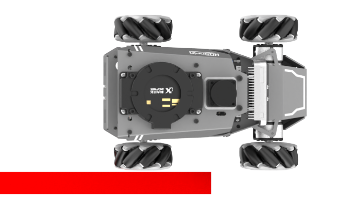
Ensure the robot is properly aligned and positioned at the start marker, then check start_test. The robot will move forward 1 meter in a straight line.
If no adjustment to the interface parameters is needed and the platform moves exactly 1 meter, the current settings are correct, as shown below.
If the robot moves more than 1 meter, the robot’s linear speed is off. Increase the odom_linear_scale_correction parameter by 0.01 at a time until the robot moves exactly 1 meter. Record this critical value, increasing it by 0.01 will cause the robot to travel less than 1 meter. If the robot moves less than 1 meter, decrease the parameter in 0.01 increments.
If there is any deviation, adjust the
odom_linear_scale_correctionvalue, which controls the scaling of the motor’s forward movement. It is recommended to change it in increments of 0.01 each time.
After calibration, open the calibration configuration file to save the corrected parameter.
cd ~/ros2_ws/src/driver/controller/config && vim calibrate_params.yaml
Press the key i to enter edit mode and modify
linear_correction_factorto the calibrated value ofodom_linear_scale_correction.
After editing, press ESC, type
:wq, and press Enter to save and exit.
2.1.4 IMU and Odometry Data Publishing
In robot navigation, calculating the real-time position is crucial.
Typically, odometry information is computed using the motor encoders combined with the robot’s kinematic model. However, in some special scenarios, such as when the robot’s wheels spin in place or the robot is lifted off the ground, it may appear that the robot has moved a certain distance, even though the wheels did not actually turn.
In such cases, fusing IMU and odometry data provides a more accurate estimation of the robot’s position, which helps improve mapping and enhances navigation accuracy.
2.1.4.1 Introduction to IMU and Odometry
The IMU, Inertial Measurement Unit, measures an object’s three-axis orientation (angular velocity) and acceleration. The gyroscope and accelerometer are the main components of the IMU, providing a total of six degrees of freedom to measure angular velocity and acceleration in 3D space.
Odometry is a method for estimating an object’s position over time based on data obtained from motion sensors. It is widely used in robotic systems to estimate how far a robot has moved relative to its initial position.
Common odometry methods include wheel odometry, visual odometry, and visual-inertial odometry. For the robot, wheel odometry is used.
The principle of wheel odometry can be illustrated with an example: Imagine you have a cart, and you want to know the distance from point A to point B.
If you know the circumference of the cart’s wheels and have a device to count the number of rotations while driving, you can calculate the distance by combining the wheel circumference with the total number of rotations during the trip from A to B.
For a wheeled robot, odometry provides a basic estimate of its pose. However, it has a significant limitation, which is cumulative error. Besides inherent hardware inaccuracies, environmental factors, such as wheel slippage caused by wet or slippery surfaces, can increase odometry errors as the robot travels farther.
Therefore, both the IMU and odometry are key components of the robot. They are used to measure the object’s three-axis orientation or angular velocity, and acceleration, as well as to estimate the robot’s displacement and pose relative to its initial position, including movement speed and direction.
To correct for errors in odometry, the IMU is used in combination, and the data from both sources are fused to obtain more accurate information.
The IMU data is published on the topic /imu, and the odometry data is published on /odom. Once both sets of data are obtained, they are fused using the ekf package in ROS, and the resulting fused localization information is then re-published.
2.1.4.2 IMU Data Publishing
Enable Service
Note
Commands must be entered with correct capitalization. The Tab key can be used to auto-complete keywords.
Power on the robot and connect it via the NoMachine remote control software. For detailed information, please refer to the section 1.7.2 AP Mode Connection Steps in the user manual.
Click the terminal icon
in the system desktop to open a command-line window.Enter the following command and press Enter to stop the app auto-start service.
sudo systemctl stop start_app_node.service
Next, enter the command and press Enter to start the chassis control node:
ros2 launch ros_robot_controller ros_robot_controller.launch.py
Open a new terminal, enter the command, and press Enter to start publishing IMU data:
ros2 launch peripherals imu_filter.launch.py
View Data
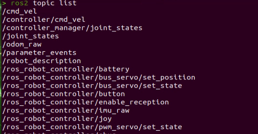
Then, open a new terminal, enter the command to check the current topics:
ros2 topic list
Next, enter the command to check the type, publisher, and subscriber of the
/imutopic. You can replace it with any topic you want to check. The type of this topic issensor_msgs/msg/Imu:
ros2 topic info /imu

Then, enter the command to print the topic message content, and you can replace it with any topic you want:
ros2 topic echo /imu
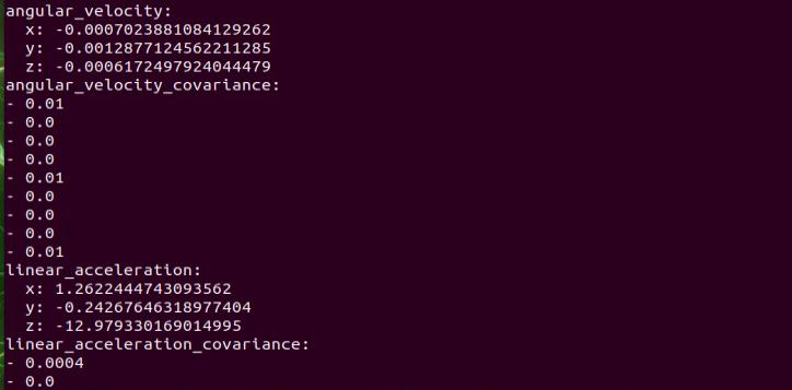
The message content shows the data collected from the three axes of the IMU.
2.1.4.3 Odometry Data Publishing
Enable Service
Note
Commands must be entered with correct capitalization. The Tab key can be used to auto-complete keywords.
Power on the robot and connect it via the NoMachine remote control software. For detailed information on connecting to a remote desktop, please refer to section 1.7.2 AP Mode Connection Steps in the user manual.
Click the terminal icon
in the system desktop to open a command-line window.Enter the following command and press Enter to stop the app auto-start service.
sudo systemctl stop start_app_node.service
Enter the command and press Enter to start publishing odometry data:
ros2 launch controller odom_publisher.launch.py
View Data
Open a new terminal, enter the command to check the current topics:
ros2 topic list
Next, enter the command to check the type, publisher, and subscriber of the
/odom_rawtopic. You can replace it with any topic you want to check. The type of this topic isnav_msgs/msg/Odometry:
ros2 topic info /odom_raw

Then, enter the command to print the topic message content. You can replace it with any topic you want:
ros2 topic echo /odom_raw
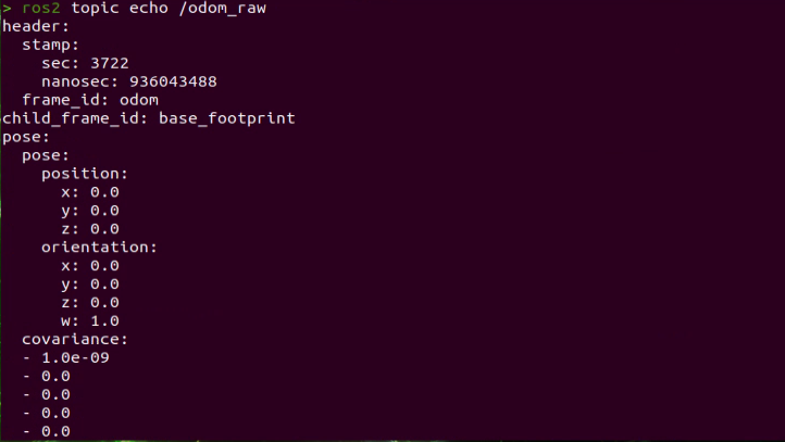
The message contains the robot’s pose and twist data.
2.1.5 Robot Speed Control
This section shows how to control the robot’s forward speed by tuning the linear velocity parameter.
2.1.5.1 Working Principle
Based on the robot’s motion characteristics, the forward, backward, and turning motions are achieved by controlling the rotation direction of the driving wheels.
The program subscribes to the /controller/cmd_vel topic to get the set linear and angular velocities, which are then used to calculate the robot’s movement speed.
2.1.5.2 Disable the App Service and Enable Speed Control
Note
Commands must be entered with correct capitalization. The Tab key can be used to auto-complete keywords.
Power on the robot and connect it to the remote control software NoMachine. For instructions on setting up the remote desktop connection, refer to the section 1.7.2 AP Mode Connection Steps in the user manual.
Click the terminal icon
in the system desktop to open a command-line window.Enter the command to stop the app service and press Enter:
sudo systemctl stop start_app_node.service
Enter the command to start the motion control service:
ros2 launch controller controller.launch.py
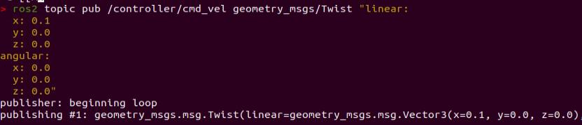
Open a new ROS2 terminal and enter the command to enable speed control:
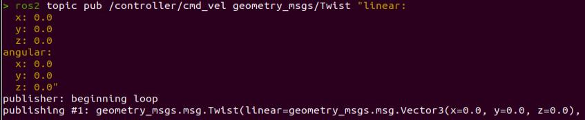
ros2 topic pub /controller/cmd_vel geometry_msgs/Twist "linear:
x: 0.0
y: 0.0
z: 0.0
angular:
x: 0.0
y: 0.0
z: 0.0"
The linear parameter sets the linear velocity. From the robot’s perspective, the positive X direction points forward, with no motion along the Y or Z axes.
The angular parameter sets the angular velocity. A positive Z value makes the robot turn left, while a negative Z value makes it turn right. There is no rotation along the X or Y axes.
Note
The unit of linear velocity X is meters per second (m/s), with a recommended range of -0.6 ~ 0.6.
Z represents the angular velocity for turning. It can be calculated using the formulas: V = ωR and tanΦA = D / R, where z = ω, D = 0.213, and ΦA is the turn angle, ranging from 0° to 36°.
Use the keyboard arrow keys to modify the corresponding parameters. For example, to move forward, set linear X to 0.1 and press Enter to execute.
To stop the robot, open a new terminal, set the previously modified linear X back to 0.0, and press Enter.
To exit this control mode, press Ctrl+C in each terminal.
Note
First, open a new terminal to stop the robot as in Step 6 before closing the control mode. If you press Ctrl+C directly in the terminal to exit, the robot may not stop properly.
2.1.5.3 Modifying Forward Speed
By adjusting the linear velocity X value, the robot can move forward at different speeds. For example, to make the robot move straight forward, set X to 0.3 as described in Step 5 of 2.1.5.2 Disable the App Service and Enable Speed Control.
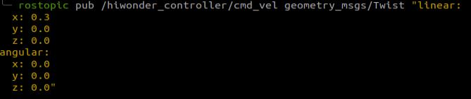
After pressing Enter, the robot will move forward at a speed of 0.3 m/s.
2.1.5.4 Program Outcome
After starting the feature, the robot will move forward at the previously set speed of 0.3 m/s.
2.1.5.5 Program Analysis
There are three files: controller.launch as the launch file, calibrate_params.yaml as the configuration file, and odom_publisher.py as the program file.
When starting, the launch file is executed first. It loads the YAML configuration file and passes the parameters to the ROS nodes. The nodes then read these parameters, initialize themselves, and communicate with other nodes to coordinate the robot’s behavior.
launch File
The launch file is located at /home/ubuntu/ros2_ws/src/driver/controller/launch/controller.launch.py
import os
from ament_index_python.packages import get_package_share_directory

from launch_ros.actions import Node
from launch.conditions import IfCondition
from nav2_common.launch import ReplaceString
from launch import LaunchDescription, LaunchService
from launch.substitutions import LaunchConfiguration
from launch.launch_description_sources import PythonLaunchDescriptionSource
from launch.actions import DeclareLaunchArgument, IncludeLaunchDescription, GroupAction, TimerAction, OpaqueFunction

def launch_setup(context):
    compiled = os.environ['need_compile']
    namespace = LaunchConfiguration('namespace', default='')
    use_namespace = LaunchConfiguration('use_namespace', default='false').perform(context)
    use_sim_time = LaunchConfiguration('use_sim_time', default='false')
    enable_odom = LaunchConfiguration('enable_odom', default='true')
    map_frame = LaunchConfiguration('map_frame', default='map')
    odom_frame = LaunchConfiguration('odom_frame', default='odom')
    base_frame = LaunchConfiguration('base_frame', default='base_footprint')
    imu_frame = LaunchConfiguration('imu_frame', default='imu_link')
    frame_prefix = LaunchConfiguration('frame_prefix', default='')

    namespace_arg = DeclareLaunchArgument('namespace', default_value=namespace)
    use_namespace_arg = DeclareLaunchArgument('use_namespace', default_value=use_namespace)
    use_sim_time_arg = DeclareLaunchArgument('use_sim_time', default_value=use_sim_time)
    enable_odom_arg = DeclareLaunchArgument('enable_odom', default_value=enable_odom)
    map_frame_arg = DeclareLaunchArgument('map_frame', default_value=map_frame)
    odom_frame_arg = DeclareLaunchArgument('odom_frame', default_value=odom_frame)
    base_frame_arg = DeclareLaunchArgument('base_frame', default_value=base_frame)
    imu_frame_arg = DeclareLaunchArgument('imu_frame', default_value=imu_frame)
    frame_prefix_arg = DeclareLaunchArgument('frame_prefix', default_value=frame_prefix)
Setting Paths
Obtain the paths for the three packages: peripherals, controller, and servo_controller.
    if compiled == 'True':
        peripherals_package_path = get_package_share_directory('peripherals')
        controller_package_path = get_package_share_directory('controller')
        servo_controller_package_path = get_package_share_directory('servo_controller')
    else:
        peripherals_package_path = '/home/ubuntu/ros2_ws/src/peripherals'
        controller_package_path = '/home/ubuntu/ros2_ws/src/driver/controller'
        servo_controller_package_path = '/home/ubuntu/ros2_ws/src/driver/servo_controller'
Starting Other Launch Files
    odom_publisher_launch = IncludeLaunchDescription(
        PythonLaunchDescriptionSource([os.path.join(controller_package_path, 'launch/odom_publisher.launch.py')
        ]),
        launch_arguments={
            'namespace': namespace,
            'use_namespace': use_namespace,
            'imu_frame': imu_frame,
            'frame_prefix': frame_prefix,
            'base_frame': base_frame,
            'odom_frame': odom_frame
        }.items()
    )
odom_publisher_launch: Launch file for odometry
imu_filter_launch IMU launch
Start Nodes
Starts the EKF fusion node.
    ekf_filter_node = Node(
        package='robot_localization',
        executable='ekf_node',
        name='ekf_filter_node',
        output='screen',
        parameters=[ekf_param, {'use_sim_time': use_sim_time}],
        remappings=[
            ('/tf', 'tf'),
            ('/tf_static', 'tf_static'),
            ('odometry/filtered', 'odom'),
            ('cmd_vel', 'controller/cmd_vel')
        ],
        condition=IfCondition(enable_odom),
    )

    servo_controller_launch = IncludeLaunchDescription(
        PythonLaunchDescriptionSource([os.path.join(servo_controller_package_path, 'launch/servo_controller.launch.py')
        ]),
        launch_arguments={
            'base_frame': base_frame,
        }.items()
    )
Python File
The Python file is located at /home/ubuntu/ros2_ws/src/driver/controller/controller/odom_publisher_node.py
Imported Libraries
#!/usr/bin/env python3
# -*- coding: utf-8 -*-
import os
import math
import time
import rclpy
import signal
import threading
from rclpy.node import Node
from std_srvs.srv import Trigger
from nav_msgs.msg import Odometry
from controller import ackermann, mecanum
from ros_robot_controller_msgs.msg import MotorsState, SetPWMServoState, PWMServoState
from geometry_msgs.msg import Pose2D, Pose, Twist, PoseWithCovarianceStamped, TransformStamped
Main Function
def main():
    node = Controller('odom_publisher')
    rclpy.spin(node)
Calls the Controller class and waits for the node to exit.
Global Parameters
ODOM_POSE_COVARIANCE = list(map(float,
                        [1e-3, 0, 0, 0, 0, 0,
                        0, 1e-3, 0, 0, 0, 0,
                        0, 0, 1e6, 0, 0, 0,
                        0, 0, 0, 1e6, 0, 0,
                        0, 0, 0, 0, 1e6, 0,
                        0, 0, 0, 0, 0, 1e3]))

ODOM_POSE_COVARIANCE_STOP = list(map(float,
                            [1e-9, 0, 0, 0, 0, 0,
                             0, 1e-3, 1e-9, 0, 0, 0,
                             0, 0, 1e6, 0, 0, 0,
                             0, 0, 0, 1e6, 0, 0,
                             0, 0, 0, 0, 1e6, 0,
                             0, 0, 0, 0, 0, 1e-9]))

ODOM_TWIST_COVARIANCE = list(map(float,
                        [1e-3, 0, 0, 0, 0, 0,
                         0, 1e-3, 0, 0, 0, 0,
                         0, 0, 1e6, 0, 0, 0,
                         0, 0, 0, 1e6, 0, 0,
                         0, 0, 0, 0, 1e6, 0,
                         0, 0, 0, 0, 0, 1e3]))

ODOM_TWIST_COVARIANCE_STOP = list(map(float,
                            [1e-9, 0, 0, 0, 0, 0,
                              0, 1e-3, 1e-9, 0, 0, 0,
                              0, 0, 1e6, 0, 0, 0,
                              0, 0, 0, 1e6, 0, 0,
                              0, 0, 0, 0, 1e6, 0,
                              0, 0, 0, 0, 0, 1e-9]))
ODOM_POSE_COVARIANCE: Odometry POSE covariance.
ODOM_POSE COVARIANCE STOP: Odometry POSE covariance when velocity is zero.
ODOM_TWIST_COVARIANCE: Odometry TWIST covariance.
ODOM_TWIST_COVARIANCE_STOP: Odometry TWIST covariance when velocity is zero.
Functions
def rpy2qua(roll, pitch, yaw):
    cy = math.cos(yaw*0.5)
    sy = math.sin(yaw*0.5)
    cp = math.cos(pitch*0.5)
    sp = math.sin(pitch*0.5)
    cr = math.cos(roll * 0.5)
    sr = math.sin(roll * 0.5)

    q = Pose()
    q.orientation.w = cy * cp * cr + sy * sp * sr
    q.orientation.x = cy * cp * sr - sy * sp * cr
    q.orientation.y = sy * cp * sr + cy * sp * cr
    q.orientation.z = sy * cp * cr - cy * sp * sr
    return q.orientation

def qua2rpy(x, y, z, w):
    roll = math.atan2(2 * (w * x + y * z), 1 - 2 * (x * x + y * y))
    pitch = math.asin(2 * (w * y - x * z))
    yaw = math.atan2(2 * (w * z + x * y), 1 - 2 * (z * z + y * y))

    return roll, pitch, yaw
rpy2qua: Converts Euler angles to a quaternion.
qua2rpy: Converts a quaternion to Euler angles.
Controller Class
(1) Call Kinematics:
        self.ackermann = ackermann.AckermannChassis(wheelbase=0.17706, track_width=0.17165, wheel_diameter=0.085)
        self.mecanum = mecanum.MecanumChassis(wheelbase=0.17706, track_width=0.17165, wheel_diameter=0.08)
self.ackermann invokes the Ackermann kinematics by initializing an Ackermann kinematics object.
(2) Define ROS Parameters:
        self.declare_parameter('pub_odom_topic', True)
        self.declare_parameter('base_frame_id', 'base_footprint')
        self.declare_parameter('odom_frame_id', 'odom')
        self.declare_parameter('linear_correction_factor', 1.00)
        self.declare_parameter('linear_correction_factor_tank', 0.52)
        self.declare_parameter('angular_correction_factor', 1.00)
        self.declare_parameter('machine_type', os.environ['MACHINE_TYPE'])


        self.pub_odom_topic = self.get_parameter('pub_odom_topic').value
        self.base_frame_id = self.get_parameter('base_frame_id').value
        self.odom_frame_id = self.get_parameter('odom_frame_id').value

        #self.machine_type = os.environ.get('MACHINE_TYPE', 'ROSOrin_Mecanum')
        self.machine_type = self.get_parameter('machine_type').value
        self.ackermann = ackermann.AckermannChassis(wheelbase=0.17706, track_width=0.17165, wheel_diameter=0.085)
        self.mecanum = mecanum.MecanumChassis(wheelbase=0.17706, track_width=0.17165, wheel_diameter=0.08)
The function self.declare_parameter is used to define a parameter.
The function self.get_parameter is used to obtain a parameter.
pub_odom_topic determines whether to publish the odometry topic.
base_frame_id specifies the robot’s base frame ID.
odom_frame_id specifies the robot’s odometry frame ID.
linear_correction_factor sets the linear velocity correction factor.
angular_correction_factor sets the angular velocity correction factor.
machine_type specifies the type of robot.
(3) Publish Odometry:
        if self.pub_odom_topic:
            # self.odom_broadcaster = tf2_ros.TransformBroadcaster(self)            # self.odom_trans = TransformStamped()
            # self.odom_trans.header.frame_id = self.odom_frame_id
            # self.odom_trans.child_frame_id = self.base_frame_id

            self.odom = Odometry()
            self.odom.header.frame_id = self.odom_frame_id
            self.odom.child_frame_id = self.base_frame_id

            self.odom.pose.covariance = ODOM_POSE_COVARIANCE
            self.odom.twist.covariance = ODOM_TWIST_COVARIANCE

            self.odom_pub = self.create_publisher(Odometry, 'odom_raw', 1)
            self.dt = 1.0/50.0

            threading.Thread(target=self.cal_odom_fun, daemon=True).start()
Whether to publish the odometry topic is determined by the pub_odom_topic parameter. If enabled, the node is initialized.
Relevant parameters are set, and the odometry is published using the self.create_publisher function. The odometry data is updated via the self.cal_odom_fun function.
(4) Topic Publishing:
        self.motor_pub = self.create_publisher(MotorsState, 'ros_robot_controller/set_motor', 1)
        self.servo_state_pub = self.create_publisher(SetPWMServoState, 'ros_robot_controller/pwm_servo/set_state', 10)
        self.pose_pub = self.create_publisher(PoseWithCovarianceStamped, 'set_pose', 1)
        self.create_subscription(Pose2D, 'set_odom', self.set_odom, 1)
        self.create_subscription(Twist, 'controller/cmd_vel', self.cmd_vel_callback, 1)
        self.create_subscription(Twist, '/app/cmd_vel', self.acker_cmd_vel_callback, 1)
        self.create_subscription(Twist, 'cmd_vel', self.app_cmd_vel_callback, 1)
        self.create_service(Trigger, 'controller/load_calibrate_param', self.load_calibrate_param)
        self.create_service(Trigger, '~/init_finish', self.get_node_state)
self.create_subscription is used to subscribe to a topic.
self.create_service is used to create a service.
self.motor_pub publishes motor control messages to ros_robot_controller/set_motor with message type MotorsState.
self.servo_state_pub publishes servo control messages to ros_robot_controller/bus_servo/set_state with message type SetBusServoState.
self.pose_pub publishes servo pose messages to set_pose with message type PoseWithCovarianceStamped.
set_odom topic publishes Pose2D messages, with the callback function self.set_odom.
controller/cmd_vel topic publishes Twist messages, with the callback function self.cmd_vel_callback.
cmd_vel topic publishes Twist messages, with the callback function self.set_app_cmd_vel_callback.
controller/load_calibrate_param service uses the Trigger type, with the callback self.load_calibrate_param.
~/init_finish service uses the Trigger type, with the callback self.get_node_state.
(5) Controller Class Function Descriptions:
get_node_state retrieves the current state of the node, used as a callback function.
load_calibrate_param reads the current motion parameters, used as a callback function.
set_odom sets the odometry values, used as a callback function.
app_cmd_vel_callback sets the robot velocity based on commands from the app, used as a callback function.
cmd_vel_callback sets the robot velocity, used as a callback function.
cal_odom_fun publishes odometry data.
2.2 Kinematics Analysis
2.2.1 Overview
The Mecanum and Ackermann robots use two fundamentally different chassis designs, each with distinct structural and motion characteristics.
2.2.1.1 Wheel Types
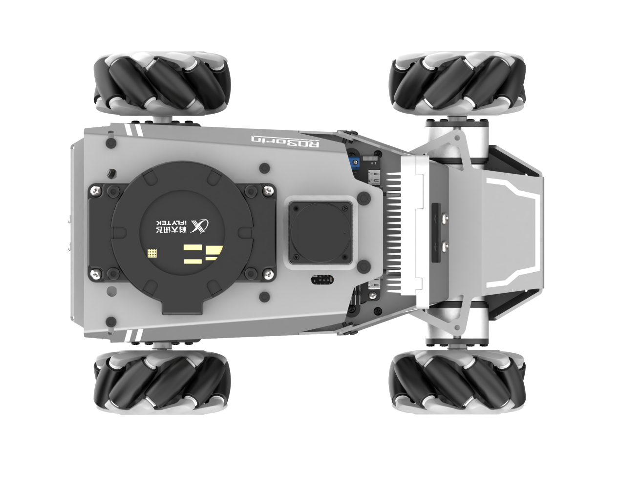
Mecanum Robot: A Mecanum chassis uses four Mecanum wheels to support the robot. Each wheel can rotate independently, and the angled rollers allow the robot to move omnidirectionally, making tight maneuvering and lateral motion possible.
Ackermann Robot: An Ackermann chassis also relies on wheels, typically with front-wheel steering and rear wheels that carry most of the robot’s weight. While the front wheels handle steering to enable turning.
Differential Robot: A differential drive chassis drives the left and right wheels independently. By varying the wheel speeds on each side, the robot can move forward, reverse, turn, or even rotate in place.
2.2.1.2 Typical Applications
Mecanum Robot: A Mecanum chassis offers exceptional maneuverability, allowing smooth and flexible turning in tight or complex environments.
Ackermann Robot: Ackermann chassis is widely used in road-driving scenarios—such as cars, trucks, and motorcycles—where steering through front wheels provides stable, predictable motion at speed.
Differential Robot: Differential drive chassis are typically used indoors or on flat surfaces because their simple layout allows for in-place turning.
2.2.2 Mecanum Chassis
2.2.2.1 Hardware Structure
A Mecanum wheel consists of a main wheel hub and multiple rollers mounted around the hub. The rollers are angled at 45 degrees relative to the axis of the hub. Typically, Mecanum wheels are used in sets of four, two left-handed wheels (Type A) and two right-handed wheels (Type B), which are arranged symmetrically.
There are several common configurations, such as AAAA, BBBB, AABB, ABAB, BABA, etc. However, not all configurations support full-range movement functions like forward/backward motion, rotation, and lateral movement. The Mecanum chassis uses the ABAB configuration, which enables true omnidirectional movement.
2.2.2.2 Physical Characteristics
The motion of a Mecanum wheel robot is determined by the direction and speed of each individual wheel. The forces generated by each wheel combine to produce a resultant force vector, allowing the robot to move freely in any desired direction without changing the orientation of the wheels.
Because of the angled rollers distributed around the edge of the wheel, lateral movement is also possible. The rollers follow a unique path. When the wheel rotates around its central axis, the roller surfaces form a cylindrical envelope, allowing the robot to roll continuously in a given direction.
The Mecanum-wheel chassis has the following main features:
1. Wheel arrangement: The chassis usually consists of four specially arranged wheels. One at each corner of the chassis, forming a diagonal pattern within a plane. This arrangement allows the robot to generate both lateral and longitudinal thrust simultaneously.
2. Rolling mechanism: Each Mecanum wheel has a unique rolling design with multiple angled rollers or beads around the circumference. These rollers enable the wheel to move in multiple directions, including sideways and forward/backward, allowing the robot to perform translational movements without changing its orientation.
3. Wheel motion control: By adjusting the speed and direction of each wheel, the robot’s movement and direction can be precisely controlled. Proper wheel control enables the vehicle to rotate, translate, or move diagonally, offering highly flexible maneuvering.
Stability: Mecanum wheels provide good stability, as the robot can move or translate in place without rotating. This is especially useful for robots navigating narrow passages or performing complex tasks.
5. Load capacity: The load capacity of Mecanum wheels depends on the design of the wheels and the drive system. They can accommodate a range of payloads, from small robots to industrial equipment.
2.2.2.3 Kinematic Principles and Equations
In kinematic analysis, the motion of Mecanum wheels can be described using a kinematic model. This includes several key parameters:
 : Linear velocity of the Mecanum chassis along the X-axis, typically the forward/backward direction.
 : Linear velocity of the Mecanum chassis along the Y-axis, typically the left/right or lateral direction.
 : Angular velocity of the Mecanum chassis, which is the rotation speed around its own center.
 : The real-time speeds of the four Mecanum wheels.
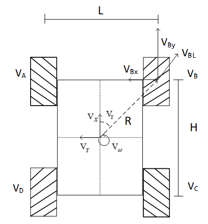
For example, the motion of the front-right wheel (Wheel B) on a 2D plane can be decomposed into:
VBx: Linear velocity of the chassis along the X-axis, typically the forward/backward direction.
VBy: Linear velocity of the chassis along the Y-axis, typically the left/right or lateral direction.
L: The distance between the centers of the left and right wheels.
H: The distance between the centers of the front and rear wheels.
 : The angle between the robot’s center of chassis and the front-right wheel is 45°.
Based on these parameters, we can perform a kinematic analysis of the Mecanum wheel chassis to determine how wheel speeds contribute to the overall movement of the robot in any direction. Key equations are given below:
Kinematic Analysis and Formula Derivation:
To simplify the kinematic model, we make the following two idealized assumptions:
(1) The Mecanum wheels do not slip on the ground, and the ground provides sufficient friction.
(2) The four wheels are positioned at the corners of a rectangle or square, and all wheels are parallel to their corresponding axes.
In this model, the robot’s rigid body movement is decomposed into three linear components: translation along the X-axis, translation along the Y-axis, and rotation around the Z-axis. By calculating the individual wheel speeds required for these three simple motions, we can combine them to compute the required rotational speed for each wheel during the compound motion of simultaneous translation and rotation.
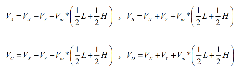
 represent the rotational speeds of wheels A, B, C, and D, respectively, corresponding to the motor speeds. is the translational velocity of the robot along the X-axis, is the translational velocity along the Y-axis, and is the rotational velocity around the Z-axis.
 is half the wheel track L, and
  is half the wheelbase H.
When the robot moves along the X-axis, the speed component of each wheel can be calculated using the following formula:
 represent the real-time speeds of the four Mecanum wheels, while represents the wheels’ speed along the X-axis.
When the robot moves along the Y-axis, the speed component of each wheel can be calculated using the following formula:
represents the speed of the Mecanum wheels along the Y-axis.
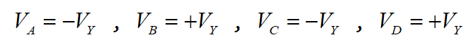
When the robot rotates around the Z-axis, the speed component of each wheel can be calculated using the following formula:
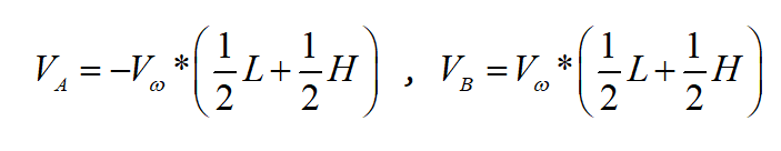
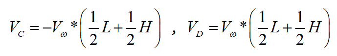
 : Angular velocity of the Mecanum chassis, which is the rotation speed around its own center.
By combining the velocities along the X, Y, and Z axes, the rotational speed required for each of the four wheels can be derived according to the robot’s overall motion state.
2.2.2.4 Program Implementation
File path: ros2_ws\src\driver\controller\controller\mecanum.py
import math
from ros_robot_controller_msgs.msg import MotorState, MotorsState

class MecanumChassis:
    # wheelbase = 0.1368   # Distance between front and real axles
    # track_width = 0.1446 # Distance between left and right axles
    # wheel_diameter = 0.065  # Wheel diameter
    def __init__(self, wheelbase=0.206, track_width=0.194, wheel_diameter=0.0065):
        self.wheelbase = wheelbase
        self.track_width = track_width
        self.wheel_diameter = wheel_diameter
Mecanum wheel kinematics class, used to calculate wheel speeds and implement the Mecanum wheel motion.
Init:
    def __init__(self, wheelbase=0.206, track_width=0.194, wheel_diameter=0.0065):
        self.wheelbase = wheelbase
        self.track_width = track_width
        self.wheel_diameter = wheel_diameter
Initializes the wheel dimensions for subsequent calculations.
speed_covert:
    def speed_covert(self, speed):
        """
        covert speed m/s to rps/s
        :param speed:
        :return:
        """
        # distance / circumference = rotations per second
        return speed / (math.pi * self.wheel_diameter)
Converts linear velocity (m/s) to angular velocity (rps/s) based on wheel parameters.
set_velocity:
    def set_velocity(self, linear_x, linear_y, angular_z):
        """
        Use polar coordinates to control moving
                    x
        v1 motor1|  ↑  |motor3 v3
          +  y - |     |
        v2 motor2|     |motor4 v4
        :param speed: m/s
        :param direction: Moving direction 0~2pi, 1/2pi<--- ↑ ---> 3/2pi
        :param angular_rate:  The speed at which the chassis rotates rad/sec
        :param fake:
        :return:
        """
        # vx = speed * math.sin(direction)
        # vy = speed * math.cos(direction)
        # vp = angular_rate * (self.wheelbase + self.track_width) / 2
        # v1 = vx - vy - vp
        # v2 = vx + vy - vp
        # v3 = vx + vy + vp
        # v4 = vx - vy + vp
        # v_s = [self.speed_covert(v) for v in [v1, v2, -v3, -v4]]
        motor1 = (linear_x - linear_y - angular_z * (self.wheelbase + self.track_width) / 2)
        motor2 = (linear_x + linear_y - angular_z * (self.wheelbase + self.track_width) / 2)
        motor3 = (linear_x + linear_y + angular_z * (self.wheelbase + self.track_width) / 2)
        motor4 = (linear_x - linear_y + angular_z * (self.wheelbase + self.track_width) / 2)
        v_s = [self.speed_covert(v) for v in [motor1, motor2, -motor3, -motor4]]
        data = []
        for i in range(len(v_s)):
            msg = MotorState()
            msg.id = i + 1
            msg.rps = float(v_s[i])
            data.append(msg)

        msg = MotorsState()
        msg.data = data
        return msg
Decomposes the input velocity parameters, computes the corresponding angular velocity using speed_covert, and publishes the resulting radian velocity to the motors.
2.2.3 Ackermann Chassis
2.2.3.1 Hardware Structure
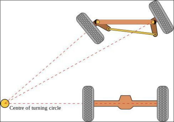
The front-wheel steering mechanism of the Ackerman chassis consists of a servo, a linkage, and the wheels. The servo connects to the linkage, which in turn connects to the wheels. By controlling the rotation of the servo, the linkage rotates accordingly, which adjusts the steering angle of the front wheels.
When the robot turns, the two front wheels remain parallel, meaning both wheels turn at the same angle. The rear wheels are driven by motors, which control the robot’s forward and backward motion as well as its speed.
2.2.3.2 Physical Characteristics
The Ackerman chassis is designed to provide excellent steering performance and stability. It employs the Ackermann geometry principle to achieve this.
The Ackermann chassis has the following main features:
1. Steering Geometry: A key feature of the Ackermann chassis is its steering geometry. By mounting the front wheels on separate steering axes, the inner and outer tires follow different turning radii during a turn. This design makes it easier for the robot to turn while reducing friction and tire wear.
2. Wheel Angles: The angles of the front wheels change with steering to match the robot’s turning radius. The inner front wheel is usually angled more than the outer front wheel to achieve better suspension performance.
3. Steering Stability: The Ackermann chassis improves robot stability and suspension performance. It helps reduce steering wobble at higher speeds and provides better control and absorption.
4. Suspension Design: The suspension system of an Ackermann chassis is typically adjusted to accommodate different front wheel steering angles, ensuring optimal suspension performance under various driving conditions.
5. Turning Radius: Because the front wheels follow different radii when turning, robots with an Ackermann chassis usually have a smaller turning radius, which is advantageous for maneuvering in tight spaces and complex paths.
2.2.3.3 Kinematic Principles and Equations
When analyzing the kinematics of an Ackerman chassis, the following mathematical parameters and formulas are used to describe its motion characteristics.
To achieve pure rolling motion, with no lateral slip when the vehicle turns, the normals of all four wheels’ rolling directions, which are the lines perpendicular to the wheel’s rolling direction, must intersect at a single point, known as the instantaneous center of rotation.
For simplicity, the model assumes only a single front wheel located at the midpoint of the front axle, as illustrated by the dashed line in the diagram. The key parameters are:
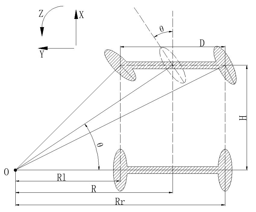
Front Wheel Steering Angle (θ): The steering angle of the front wheel relative to the vehicle’s forward direction, typically measured in radians (rad).
Vehicle Linear Velocity (V): The translational speed of the vehicle, measured in meters per second (m/s). Left rear wheel speed: VL. Right rear wheel speed: VR.
Wheel Track (D): The distance between the left and right wheels, measured in meters (m).
Wheelbase (H): The distance between the front and rear wheels, measured in meters (m).
Turning Radius (R): The radius of the circular path followed by the vehicle when turning, measured in meters (m).
Left wheel turning radius: RL. Right wheel turning radius: RR.
Computation of robot velocity and wheel speeds:
Angular velocity consistency:
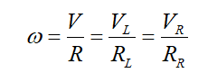
ω is the angular velocity of the robot, R is the turning radius of the robot’s center, V is the linear velocity of the robot, VL and VR are the linear velocities of the left and right rear wheels, and RL and RR are their respective turning radii.
Relationship between the front wheel steering angle and the turning radius:
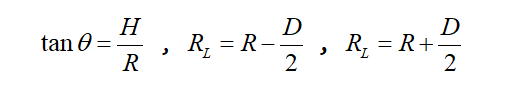
H is the wheelbase, R is the turning radius of the robot, D is the track width, and θ is the steering angle of the front wheel, where H is the distance between the front and rear axles, and D is the distance between the left and right wheels.
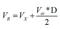
Left rear wheel velocity:
Right rear wheel velocity:
Given the robot’s track width, wheelbase, linear velocity, and steering angle, the velocities of the left and right rear wheels can be determined.
2.2.3.4 Program Implementation
File path: ros2_ws\src\driver\controller\controller\ackermann.py
class AckermannChassis:
    # wheelbase = 0.213  # Distance between front and real axles
    # track_width = 0.222  # Distance between left and right axles
    # wheel_diameter = 0.101  # Wheel diameter

    def __init__(self, wheelbase=0.213, track_width=0.222, wheel_diameter=0.101):
        self.wheelbase = wheelbase
        self.track_width = track_width
        self.wheel_diameter = wheel_diameter
Ackerman Kinematics class, used to compute wheel velocities and implement Ackerman steering kinematics.
Init:
    def __init__(self, wheelbase=0.213, track_width=0.222, wheel_diameter=0.101):
        self.wheelbase = wheelbase
        self.track_width = track_width
        self.wheel_diameter = wheel_diameter
Initializes the wheel dimensions for subsequent calculations.
speed_covert:
    def speed_covert(self, speed):
        """
        covert speed m/s to rps/s
        :param speed:
        :return:
        """
        return speed / (math.pi * self.wheel_diameter)
Converts linear velocity (m/s) to angular velocity (rps/s) based on wheel parameters.
set_velocity:
    def set_velocity(self, linear_speed, angular_speed, reset_servo=True):
        servo_angle = 1500
        data = []
        if abs(linear_speed) >= 1e-8:
            if abs(angular_speed) >= 1e-8:
                theta = math.atan(self.wheelbase*angular_speed/linear_speed)
                steering_angle = theta
                # print(math.degrees(steering_angle))
                if steering_angle > math.radians(34):
                    steering_angle = math.radians(34)
                elif steering_angle < math.radians(-34):
                    steering_angle = math.radians(-34)
                servo_angle = 1500 + 2000*math.degrees(-steering_angle)/180

            vr = linear_speed + angular_speed*self.track_width/2
            vl = linear_speed - angular_speed*self.track_width/2
            v_s = [self.speed_covert(v) for v in [0, vl, 0, -vr]]
            for i in range(len(v_s)):
                msg = MotorState()
                msg.id = i + 1
                msg.rps = float(v_s[i])
                data.append(msg)
            msg = MotorsState()
            msg.data = data
            return servo_angle, msg
        else:
            for i in range(4):
                msg = MotorState()
                msg.id = i + 1
                msg.rps = 0.0
                data.append(msg)
            msg = MotorsState()
            msg.data = data
Decomposes the input velocity parameters, converts them into wheel speeds using speed_covert, and publishes the computed angular velocities to the motors. Based on the linear and angular velocities, it calculates the required steering angle for the servo and sends the converted value to the servo for execution.