6. Machine Learning Application

6.1 YOLOv11 Model

6.1.1 Introduction to the YOLO Series of Models

6.1.1.1 YOLO Series

YOLO (You Only Look Once) is a One-stage, deep learning-based regression approach to object detection.

Before the advent of YOLOv1, the R-CNN family of algorithms dominated the object detection field. Although the R-CNN series achieved high detection accuracy, its Two-stage architecture limited its speed, making it unsuitable for real-time applications.

To address this issue, the YOLO series was developed. The core idea behind YOLO is to redefine object detection as a regression problem. It processes the entire image as input to the network and directly outputs Bounding Box coordinates along with their corresponding class labels. Compared to traditional object detection methods, YOLO offers faster detection speed and higher average precision.

6.1.1.2 YOLOv11

YOLOv11 builds upon previous versions of the YOLO model, delivering significant improvements in both detection speed and accuracy.

A typical object detection algorithm can be divided into four modules: the input module, the backbone network, the neck network, and the head output module. Analyzing Yolov11 according to these modules reveals the following enhancements:

1. Input: Added adaptive grayscale filling and dynamic Mosaic enhancement, optimizing adaptability and training efficiency.

2. Backbone Network: Utilizes the C3K2 module, which combines 1×1, 3×3, and 5×5 multi-scale convolution kernels to expand the receptive field while reducing computational load, along with the GSConv+GWGA combination.

3. Neck Network: Based on the FPN+PAN framework, the C2PSA module is inserted.

4. Head Output Layer: Adopts a classification-regression decoupled head, with the classification head focusing on semantic features and the regression head focusing on location features, and introduces dynamic head weight adjustment where weights are dynamically allocated between the two heads based on the loss during training to improve overall performance.

6.1.2 Yolov11 Model Structure

6.1.2.1 Components

1. Convolutional Layer: Feature Extraction

Convolution is the process where an entity at multiple past time points does or is subjected to the same action, influencing its current state. Convolution can be divided into convolution and multiplication.

Convolution can be understood as flipping the data, and multiplication as the accumulation of the influence that past data has on the current data. The data flipping is done to establish relationships between data points, facilitating the calculation of accumulated influence with a proper reference.

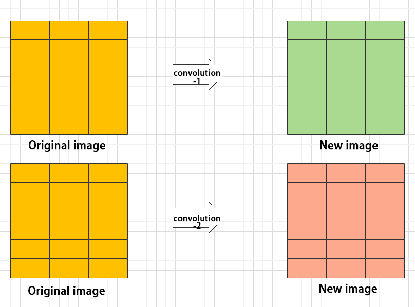
In Yolov11, the data to be processed are images, which are two-dimensional in computer vision. Accordingly, the convolution is a two-dimensional convolution. The purpose of 2D convolution is to extract features from images. To perform a 2D convolution, it is necessary to understand the convolution kernel.

The convolution kernel is the unit region over which the convolution calculation is performed each time. The unit is pixels, and the convolution sums the pixel values within the region. Typically, convolution is done by sliding the kernel across the image, and the kernel size is manually set.

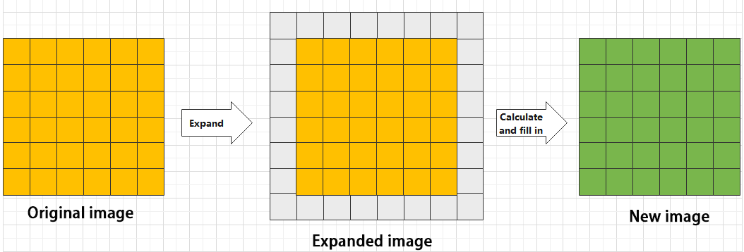
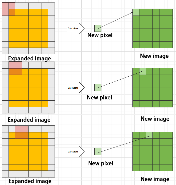
When performing convolution, depending on the desired effect, the image borders may be padded with zeros or extended by a certain number of pixels, then the convolution results are placed back into the corresponding positions in the image. For example, a 6×6 image is first expanded to 7×7, then convolved with the kernel, and finally the results are filled back into a blank 6×6 image.

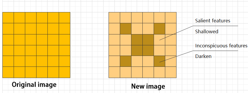
2. Pooling Layer: Feature Amplification

The pooling layer, also called the downsampling layer, is usually used together with convolution layers. After convolution, pooling performs further sampling on the extracted features. Pooling includes various types such as global pooling, average pooling, max pooling, etc., each producing different effects.

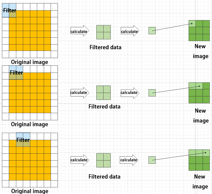
To make it easier to understand, max pooling is used here as an example. Before understanding max pooling, it is important to know about the filter, which is like the convolution kernel—a manually set region that slides over the image and selects pixels within the area.

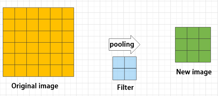
Max pooling keeps the most prominent features and discards others. For example, starting with a 6×6 image, applying a 2×2 filter for max pooling produces a new image with reduced size.

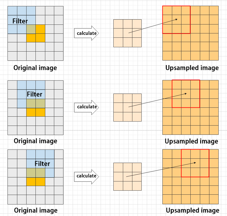
3. Upsampling Layer: Restoring Image Size

Upsampling can be understood as “reverse pooling.” After pooling, the image size shrinks, and upsampling restores the image to its original size. However, only the size is restored, the pooled features are also modified accordingly.

For example, starting with a 6×6 image, applying a 3×3 filter for upsampling produces a new image.

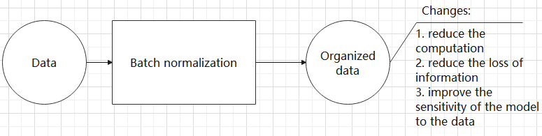
4. Batch Normalization Layer: Data Regularization

Batch normalization means rearranging the data neatly, which reduces the computational difficulty of the model and helps map data better into the activation functions.

Batch normalization reduces the loss rate of features during each calculation, retaining more features for the next computation. After multiple computations, the model’s sensitivity to the data increases.

5. ReLU Layer: Activation Function

Activation functions are added during model construction to introduce non-linearity. Without activation functions, each layer is essentially a matrix multiplication. Every layer’s output is a linear function of the previous layer’s input, so no matter how many layers the neural network has, the output is just a linear combination of the input. This prevents the model from adapting to actual situations.

There are many activation functions, commonly ReLU, Tanh, Sigmoid, etc. Here, ReLU is used as an example. ReLU is a piecewise function that replaces all values less than 0 with 0 and keeps positive values unchanged.

6. ADD Layer: Tensor Addition

Features can be significant or insignificant. The ADD layer adds feature tensors together to enhance the significant features.

7. Concat Layer: Tensor Concatenation

The Concat layer concatenates feature tensors to combine features extracted by different methods, thereby preserving more features.

6.1.2.2 Composite Elements

When building a model, using only the basic layers mentioned earlier can lead to overly lengthy, disorganized code with unclear hierarchy. To improve modeling efficiency, these basic elements are often grouped into modular units for reuse.

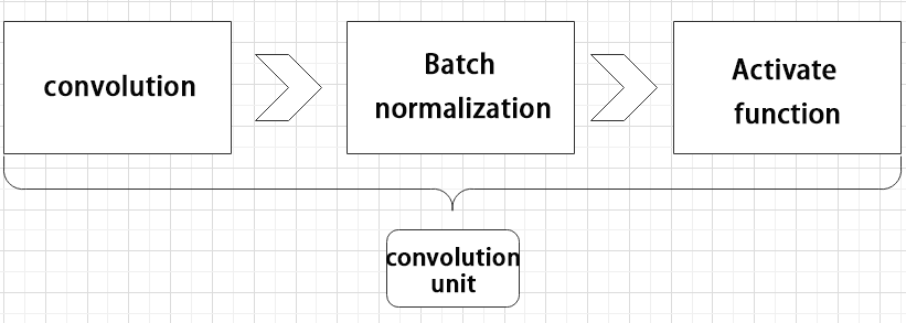
1. Convolutional Block

A convolutional block consists of a convolutional layer, a batch normalization layer, and an activation function. The process follows this order: convolution → batch normalization → activation.

2. Strided Sampling and Concatenation Unit（Focus）

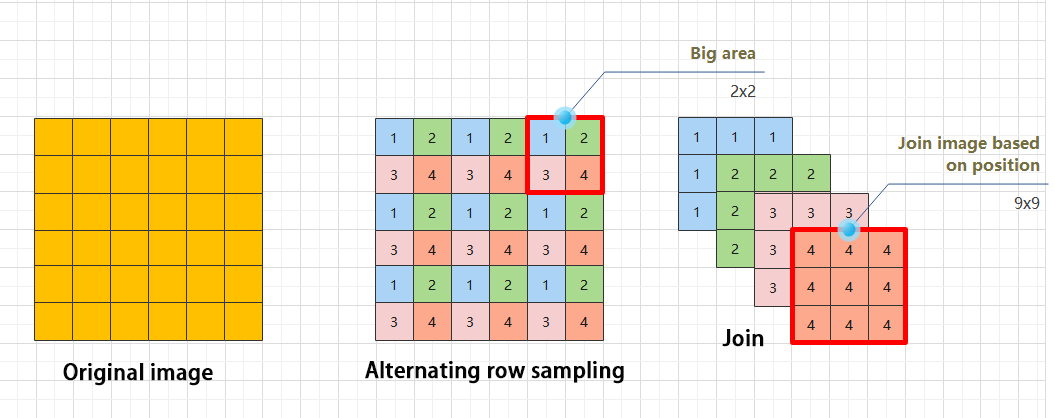
The input image is first divided into multiple large regions. Then, small image patches located at the same relative position within each large region are concatenated together to form a new image. This effectively splits the input image into several smaller images. Finally, an initial sampling is performed on the images using a convolutional block.

As shown in the figure below, for a 6×6 image, if each large region is defined as 2×2, the image can be divided into 9 large regions, and each contains 4 small patches.

By taking the small patches at position 1 from each large region and concatenating them, a 3×3 image can be formed. The patches at other positions are concatenated in the same way.
Ultimately, the original 6×6 image is decomposed into four 3×3 images.

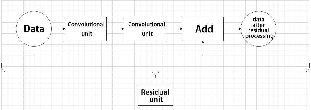
3. Residual Block

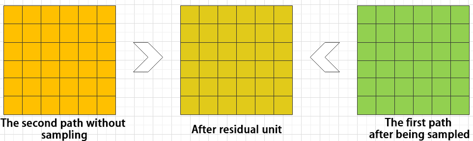
The residual block enables the model to learn subtle variations in the image. Its structure is relatively simple and involves merging data from two paths.

In the first path, two convolutional blocks are used to extract features from the image. In the second path, the original image is passed through directly without convolution. Finally, the outputs from both paths are added together to enhance learning.

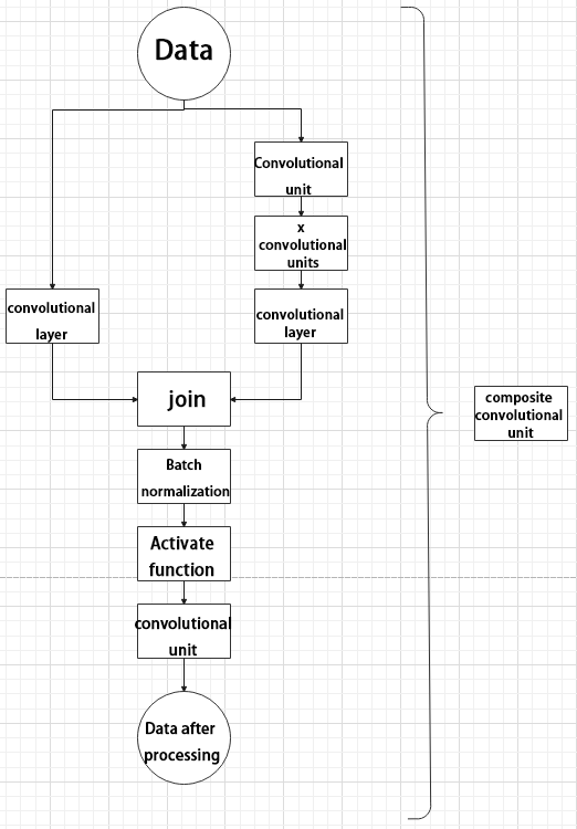
4. Composite Convolutional Block

In Yolov11, a key feature of the composite convolutional block is its customizable design, allowing convolutional blocks to be configured as needed. This structure also uses two paths whose outputs are merged.

The first path contains a single convolutional layer for feature extraction, while the second path includes 2𝑥+1 convolutional blocks followed by an additional convolutional layer. After sampling and concatenation, batch normalization is applied to standardize the data, followed by an activation function. Finally, a convolutional block is used to process the combined features.

5. Composite Residual Convolutional Block

The composite residual convolutional block modifies the composite convolutional block by replacing the 2𝑥 convolutional blocks with 𝑥 residual blocks. In Yolov11, this block is also customizable, allowing residual blocks to be tailored according to specific requirements.

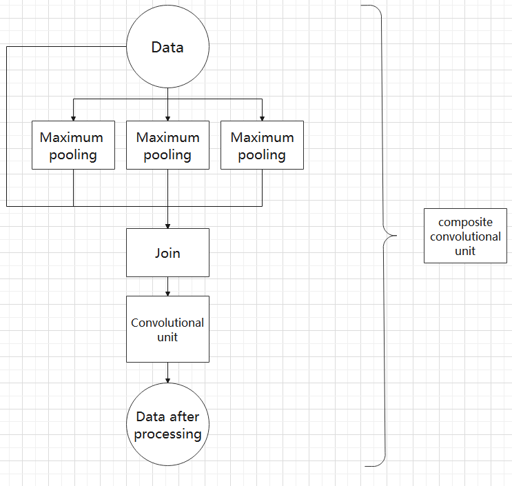
6. Composite Pooling Block

The output from a convolutional block is simultaneously passed through three separate max pooling layers, while an additional unprocessed copy is preserved. The resulting four feature maps are then concatenated and passed through a convolutional block. By processing data with the composite pooling block, the original features can be significantly enhanced and emphasized.

6.2 Yolov11 Workflow

This section explains the model’s processing flow using the concepts of prior boxes, prediction boxes, and anchor boxes involved in Yolov11.

6.2.1 Prior Box

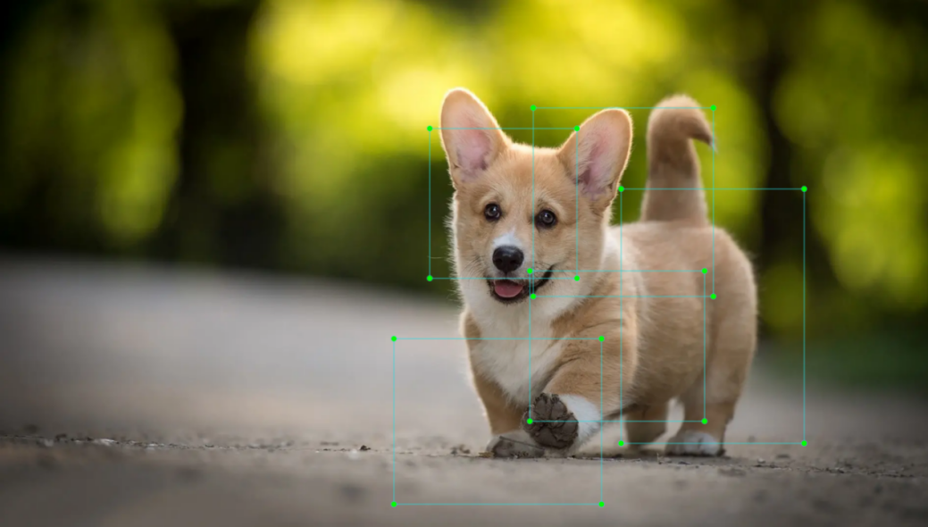
When an image is fed into the model, predefined regions of interest must be specified. These regions are marked using prior boxes, which serve as initial bounding box templates indicating potential object locations in the image.

6.2.2 Predicted Box

Prediction boxes are generated by the model as output and do not require manual input. When the first batch of training data is fed into the model, the prediction boxes are automatically created. The center points of prediction boxes tend to be located in areas where similar objects frequently appear.

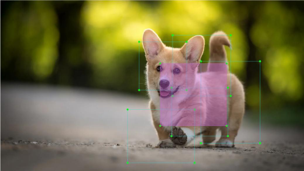
6.2.3 Anchor Box

Since predicted boxes may have deviations in size and location, anchor boxes are introduced to correct these predictions.

Anchor boxes are positioned based on the predicted boxes. By influencing the generation of subsequent predicted boxes, anchor boxes are placed around their relative centers to guide future predictions.

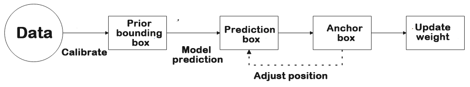
6.2.4 Project Process

Once the bounding box annotations are complete, prior boxes appear on the image. When the image data is input into the model, predicted boxes are generated based on the locations of the prior boxes. Subsequently, anchor boxes are generated to adjust the predicted results. The weights from this round of training are then updated in the model.

With each new training iteration, the predicted boxes are influenced by the anchor boxes from the previous round. This process is repeated until the predicted boxes gradually align with the prior boxes in both size and location.

6.3 Image Collection and Annotation

Training the Yolov11 model requires a large amount of data, so data collection and annotation must be performed first to prepare for model training.

In this example, the demonstration uses traffic signs as target objects.

6.3.1 Image Collection

1. Power on the robot and connect it to a remote control tool like VNC.

2. Click the terminal icon in the system desktop to open a command-line window.

3. Stop the app auto-start service by entering the following command:

~/.stop_ros.sh

4. Start the monocular camera service with command:

ros2 launch peripherals usb_cam.launch.py

5. Open a new command-line terminal and enter the command to create a directory for storing your dataset.

mkdir -p ~/my_data

6. Then, launch the tool by entering the following command.

cd ~/software/collect_picture && python3 main.py

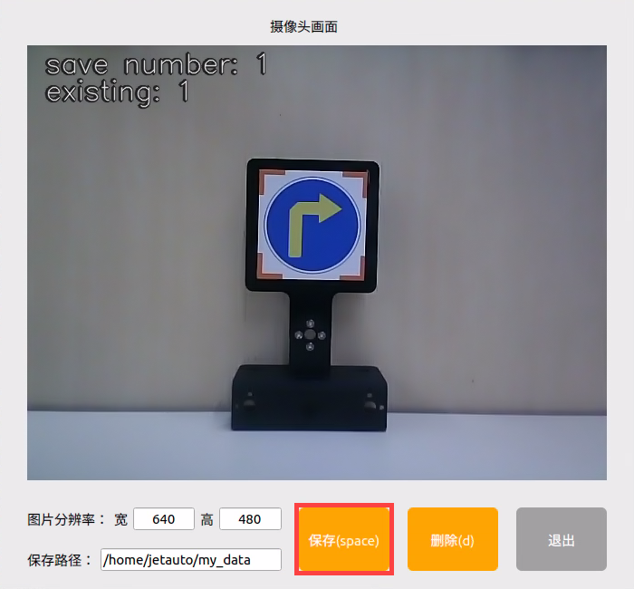
The save number in the top-left corner of the tool interface shows the ID of the saved image. The existing shows how many images have already been saved.

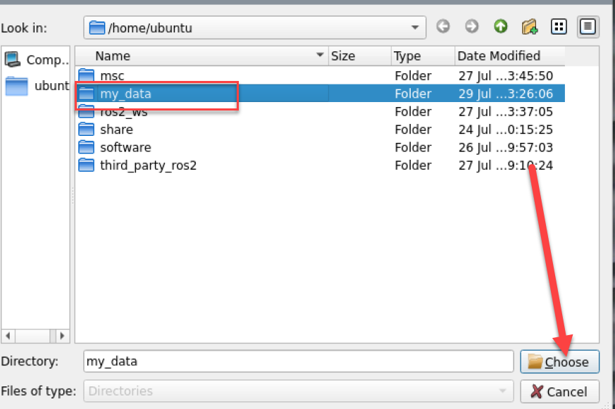
7. Click Choose to change the save path to the my_data folder created before.

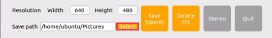
8. After selecting the target directory, click Choose.

9. Place the target object within the camera view and click the Save(space) button or press the spacebar to save the current camera frame.

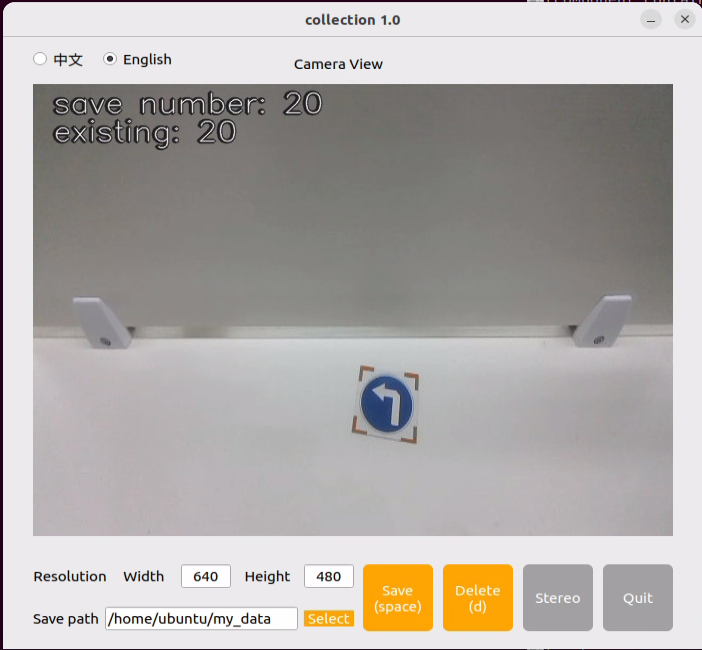
After pressing Save(space) or the spacebar, a folder named JPEGImages will be automatically created under the path /home/ubuntu/my_data to store the images.

Note

To improve model reliability, capture the target object from various distances, angles, and tilts.

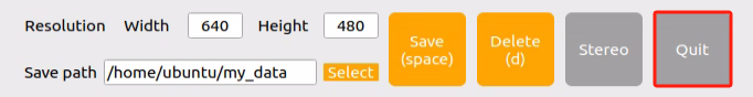
10. After collecting images, click the Quit button to close the tool.

11. Then press Ctrl+C in all opened terminal windows to exit. This completes the image collection process.

6.3.2 Image Annotation

Once the images are collected, they need to be annotated. Annotation is essential for creating a functional dataset, as it tells the training model which parts of the image correspond to which categories. This allows the model to later identify those categories in new, unseen images.

Note

When entering commands, make sure to use correct case and spacing. The Tab key can be used to auto-complete keywords.

1. Open a terminal and enter the command to start the image annotation tool:

python3 ~/software/labelImg/labelImg.py

Below is a table of common shortcut keys:

Button	Shortcut Key	Function
	Ctrl+U	Choose the directory for images.
	Ctrl+R	Choose the directory for calibration data.
	W	Create an annotation box.
	Ctrl+S	Save the annotation.
	A	Switch to the previous image.
	D	Switch to the next image.

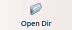
2. Click the button to open the folder where your images are stored. In this tutorial, select the directory used for image collection.

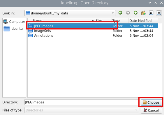
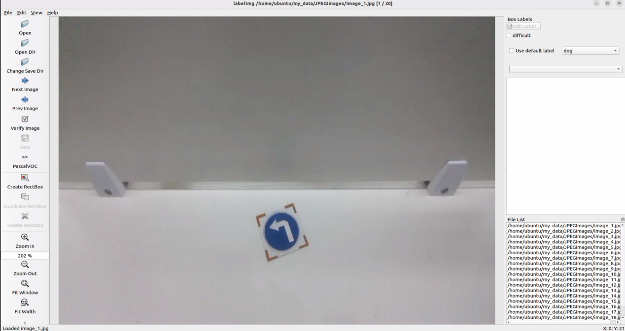
3. The folder opens the interface shown below.

4. Then click the Change Save Dir button and select the annotation save folder, which is the Annotations directory located under the same path as the image collection.

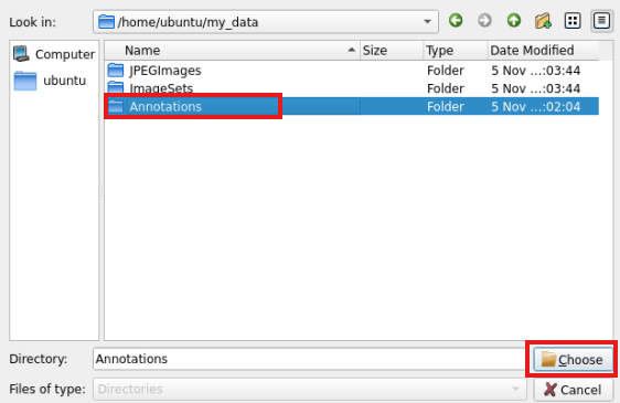
5. Click Choose to return to the annotation interface.

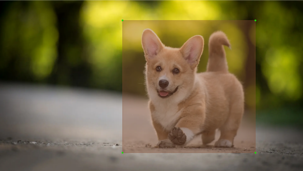
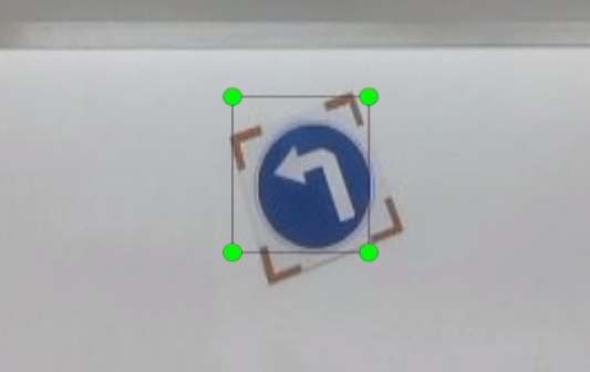
6. Press the W key to begin creating a bounding box.

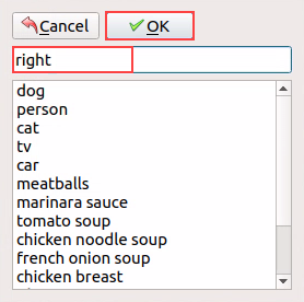
7. Move the mouse to the desired location and hold the left mouse button to draw a box that covers the entire object. Release the left mouse button to finish drawing the box.

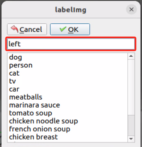
8. In the pop-up window, name the category of the object, e.g., left. After naming, click OK or press Enter to save the label.

9. Press Ctrl+S to save the annotation for the current image.

10. Press the D key to move to the next image, then repeat steps 7 to 9 to complete all annotations. Click the close button at the top-right corner of the tool to exit.

11. Open a new terminal and enter the following command to view the annotation files:

cd my_data/Annotations && ls

6.4 Data Format Conversion

6.4.1 Preparation

Before starting the operations in this section, image collection and annotation must be completed first. For detailed steps, refer to the section Image Collection and Annotation.

Before training the Yolov11 model with the data, the images need to be assigned categories, and the annotation data must be converted into the proper format.

6.4.2 Data Format Conversion

Before starting the operations in this section, image collection and annotation must be completed first.

Note

When entering commands, make sure to use correct case and spacing. The Tab key can be used to auto-complete keywords.

1. Open a new terminal and enter the following command to open the file:

Note

Create a file if the file cannot be found.

vim ~/my_data/classes.names

2. Press the i key, and enter the annotated class name left in the file. If there are multiple categories, each one should be listed on a new line.

3. After editing, press Esc, type the command :wq, and press Enter to save and exit.

Note

The class names here must match the labels used in the labelImg annotation tool exactly.

4. Next, return to the terminal and run the following command to convert the annotation format:

python3 ~/software/yolov11/xml2yolo.py --data ~/my_data --yaml ~/my_data/data.yaml

Note

Make sure the path to my_data matches the actual file structure!

This command uses three main parameters:

1. xml2yolo.py: A script that converts annotations from XML format to the YOLOv11 format. Make sure the path is correct.

2. my_data: The directory containing the annotated dataset.

3. data.yaml: A YAML file that specifies how the dataset is split and configured for training. It will be saved inside the my_data folder.

The following image shows a generated example of data.yaml:

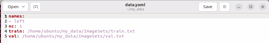
The items listed after the names represent the types of labels. The nc field specifies the total number of label categories. The train refers to the training set—a commonly used term in deep learning that indicates the data used for model training. The parameter following it is the path to the training images. Similarly, the val refers to the validation set, which is used to verify the model’s performance during the training process, and the path that follows indicates where the validation data is located. These file paths need to be set based on the actual location of your data. For example, to speed up the training process later by moving the dataset from the robot to a local PC or a cloud server, the train and val paths should be updated accordingly to reflect their new locations.

Finally, an XML file will be generated under the ~/my_data folder to record the path location of the currently split dataset. Similarly, the last parameter in step 4, ~/my_data/data.yaml, can be changed to modify the save path. This file path must be remembered, as it will be used later for model training.

6.5 Model Training

Note

When entering commands, make sure to use correct case and spacing. The Tab key can be used to auto-complete keywords.

6.5.1 Preparation

After the model format conversion is complete, proceed to the model training stage. Before training, ensure that the dataset has already been converted to the required format. For details, refer to Section 6.4 Data Format Conversion in this document.

6.5.2 Model Training

1. Power on the robot and connect it to a remote control tool like VNC.

2. Click the terminal icon in the system desktop to open a command-line window.

3. Enter the following command and press Enter to go to the specific directory.

cd ~/software/yolov11

4. Enter the command to start training the model.

python3 train.py --img 640 --batch 64 --epochs 300 --data ~/my_data/data.yaml --weights yolo11n.pt

In the command, the parameters stands for:
–img: image size.
–batch: number of images per batch.
–epochs: number of training iterations.
–data: path to the dataset.
–weights: path to the pre-trained model.

The above parameters can be adjusted according to the specific setup. To improve model accuracy, consider increasing the number of training epochs. Note that this will also increase training time.

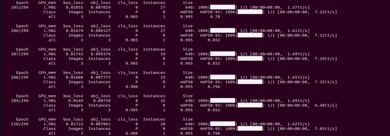
If the following content appears, it indicates that the training is in progress.

After training is complete, the terminal will display the path where the trained model files are saved. The training results are stored in the directory of /home/ubuntu/runs/detect/train/weights.

Note

The generated folder name under runs/detect may vary. Please locate it accordingly.

6.6 Traffic Sign Model Training

Note

The product names and reference paths mentioned in this document may vary. Please refer to the actual setup for accurate information.

When dealing with large datasets, it is not recommended to train models directly on the robot’s onboard motherboard due to I/O speed and memory limitations. Instead, it is advised to use a PC with a dedicated GPU, which follows the same training steps, only requiring proper environment configuration.

In the following instructions, screenshots may show different robot hostnames, as different robots have similar environment setups. Simply follow the command steps in the document as described — it does not affect the execution.

6.6.1 Preparation

1. Prepare a laptop, or if using a desktop, make sure to have a wireless network card, mouse, and other necessary tools.

2. Use the previously learned method to install and open the remote control tool VNC.

6.6.2 Operation Steps

6.6.2.1 Image Collection

1. Power on the robot and connect it to a remote control tool like VNC.

2. Click the terminal icon in the system desktop to open a command-line window.

3. Execute the following command to stop the app service:

~/.stop_ros.sh

4. Enter the following command to create a new directory for storing the dataset:

mkdir -p ~/my_data

5. Execute the following command to start the camera service:

ros2 launch peripherals usb_cam.launch.py

6. Open a new terminal, navigate to the image collection tool directory, and run the image collection script:

cd software/collect_picture && python3 main.py

The save number in the top-left corner of the tool interface shows the ID of the saved image. The existing shows how many images have already been saved.

7. Change the save path to /home/ubuntu/my_data, which will also be used in later steps.

8. Place the target object within the camera’s view. Press the Save(space) button or the spacebar to save the current camera frame. After pressing it, both the save number and the existing counters will increase by 1. This helps track the current image ID and total image count in the folder.

After clicking Save (space), a folder named JPEGImages will be automatically created under the path /home/ubuntu/my_data to store the images.

Note

To improve model reliability, capture the target object from various distances, angles, and tilts. To ensure stable recognition, collect at least 200 images per category during the data collection phase.

9. After collecting images, click the Quit button to close the tool.

6.6.2.2 Image Annotation

Note

When entering commands, make sure to use correct case and spacing. The Tab key can be used to auto-complete keywords.

1. Power on the robot and connect it to a remote control tool like VNC.

2. Click the terminal icon in the system desktop to open a command-line window.

3. Execute the following command to stop the app service:

~/.stop_ros.sh

4. Open a new terminal and enter the following command.

python3 software/labelImg/labelImg.py

5. After opening the image annotation tool. Below is a table of common shortcut keys:

Button	Shortcut Key	Function
	Ctrl+U	Choose the directory for images.
	Ctrl+R	Choose the directory for calibration data.
	W	Create an annotation box.
	Ctrl+S	Save the annotation.
	A	Switch to the previous image.
	D	Switch to the next image.

6. Use the shortcut Ctrl+U, set the image storage directory to /home/ubuntu/my_data/JPEGImages/, and click Choose.

7. Use the shortcut Ctrl+R, set the annotation data storage directory to /home/ubuntu/my_data/Annotations/, and click Choose. The Annotations folder will be automatically generated when collecting images.

8. Press the W key to begin creating a bounding box.

Move the mouse to the desired location and hold the left mouse button to draw a box that covers the entire object. Release the left mouse button to finish drawing the box.

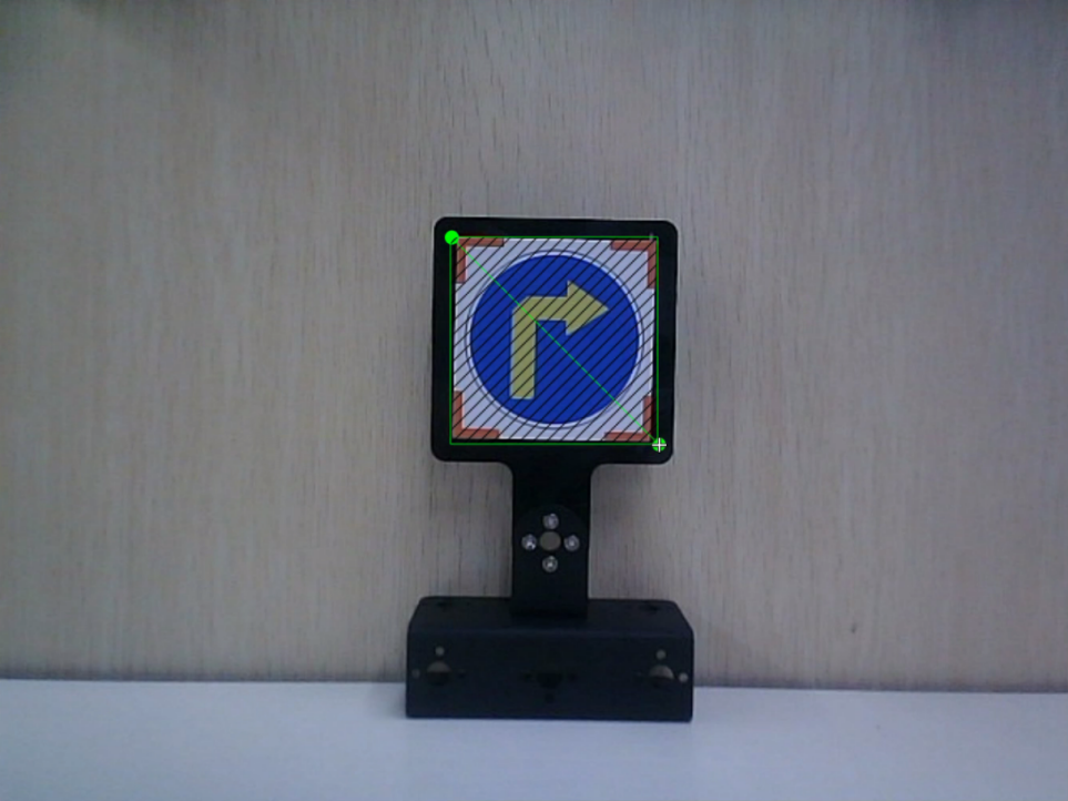
9. In the pop-up window, name the category of the object, e.g., right. After naming, click OK or press Enter to save the label.

10. Press Ctrl+S to save the annotation for the current image.

11. Refer to Step 9 to complete the annotation of the remaining images.

12. Navigate to the directory /home/ubuntu/my_data/Annotations/. This is the same dataset path where the images were saved during data collection. The annotation files corresponding to each image can be viewed in this folder.

6.6.2.3 Generating Related Files

1. Click the terminal icon in the system desktop to open a command-line window.

2. Enter the following command to open the file for editing:

vim ~/my_data/classes.names

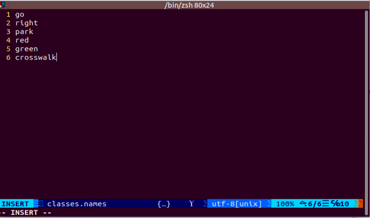
3. Press the i key to enter edit mode and add the class names for the target recognition objects. When adding multiple class names, each class name should be listed on a separate line.

Note

4. After editing, press Esc, then type :wq to save and close the file.

5. Next, enter the command to convert the data format and press Enter:

python3 ~/software/yolov11/xml2yolo.py --data ~/my_data --yaml ~/my_data/data.yaml

In this command, the xml2yolo.py file is used to convert the annotated files into XML format and categorize the dataset into training and validation sets.

The output paths depend on the actual storage location of the folders in the robot’s file system. Paths may vary across devices, but the generated data.yaml file will correspond to your annotated dataset.

6.6.2.4 Model Training

1. Click the terminal icon in the system desktop to open a command-line window.

2. Then enter the command to navigate to the specific directory.

cd ~/software/yolov11

3. Enter the command to start training the model.

python3 train.py --img 640 --batch 64 --epochs 300 --data ~/my_data/data.yaml --weights yolo11n.pt

In the command, –img specifies the image size, –batch indicates the number of images input per batch, –epochs refers to the number of training iterations, representing how many times the machine learning model will go through the dataset. This value should be optimized based on the actual performance of the final model. If the computer system is more powerful, this value can be increased to achieve better training results. –data is the path to the dataset, which refers to the folder containing the manually annotated data. –weights indicates the path to the pre-trained model weights. This specifies which .pt weight file the training process is based on. It’s important to note whether yolo11n.pt, yolo11s.pt, or another version is used.

The above parameters can be adjusted according to the specific setup. To improve model accuracy, consider increasing the number of training epochs. Note that this will also increase training time.

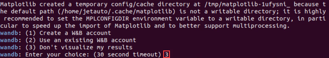
4. When the following options appear as shown in the image, enter 3 and press Enter.

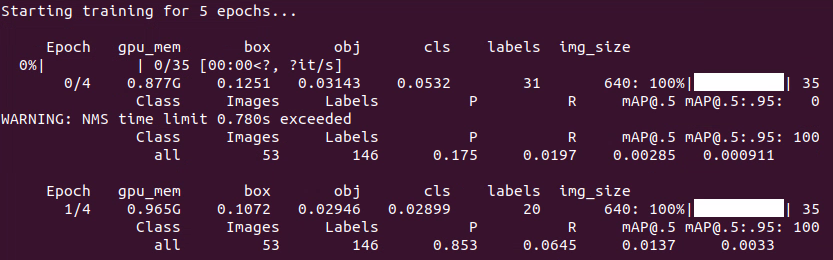
If the following content appears, it indicates that the training is in progress.

After the model training is completed, the terminal will print the path where the output files are saved. Please make sure to record this path.

6.6.3 Using the Model

1. Open the terminal , enter the following command, and press Enter to disable the app auto-start service.

~/.stop_ros.sh

2. Enter the following command to navigate to the directory where the corresponding feature’s program is located:

cd /home/ubuntu/software/yolov11

3. Enter the command to view the models in the current directory. Pretrained models are already provided, as shown below.

The content in the red box, where best_traffic.pt is the trained best.pt model. Other trained models can be added to this directory as needed.

ls

4. Next, enter the command to check the program that calls the model, and manually modify the model name.

vim ~/ros2_ws/src/yolov11_detect/yolov11_detect/yolov11_detect_demo.py

5. Change MODEL_DEFAULT_NAME to best_traffic, and then type :wq to save and exit.

6. Navigate to the ROS2 workspace, then compile the project and wait for the build to complete.

cd ~/ros2_ws

colcon build --event-handlers console_direct+ --cmake-args -DCMAKE_BUILD_TYPE=Release --symlink-install --packages-select yolov11_detect

7. After the compilation is complete, open a new command-line terminal , enter the command, and run the model execution program.

ros2 launch yolov11_detect yolov11_detect_demo.launch.py