12 ROS1-MoveIt & Gazebo Simulation

12.1 URDF Model Introduction V1.0

12.1.1 URDF Model

URDF Model Introduction

The Unified Robot Description Format (URDF) is an XML file format widely used in ROS (Robot Operating System) to comprehensively describe all components of a robot.

Robots are typically composed of multiple links and joints. A link is defined as a rigid object with certain physical properties, while a joint connects two links and constrains their relative motion.

By connecting links with joints and imposing motion restrictions, a kinematic model is formed. The URDF file specifies the relationships between joints and links, their inertial properties, geometric characteristics, and collision models.

Comparison between Xacro and URDF Model

The URDF model serves as a description file for simple robot models, offering a clear and easily understandable structure. However, when it comes to describing complex robot structures, using URDF alone can result in lengthy and unclear descriptions.

To address this limitation, the xacro model extends the capabilities of URDF while maintaining its core features. The xacro format provides a more advanced approach to describe robot structures. It greatly improves code reusability and helps avoid excessive description length.

For instance, when describing the two legs of a humanoid robot, the URDF model would require separate descriptions for each leg. On the other hand, the xacro model allows for describing a single leg and reusing that description for the other leg, resulting in a more concise and efficient representation.

Install URDF Dependencies

Note

Note: The URDF model and Xacro model are already installed in both the robot and the virtual machine. Users do not need to reinstall them. The information provided in this section is solely for comprehension purposes.

Run the command ‘sudo apt update’, and hit Enter key to update the installation package info.
```
sudo apt update
```
Execute the command ‘sudo apt-get install ros-melodic-urdf’, and hit Enter to install URDF dependency.
```
sudo apt-get install ros-melodic-urdf
```

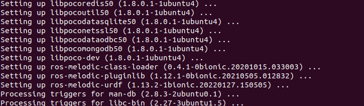
When you receive the following messages, it means the dependencies are installed successfully.

Type the command ‘sudo apt-get install ros-melodic-xacro’, and hit Enter key to install URDF model extension format: Xacro.
```
sudo apt-get install ros-melodic-xacro
```

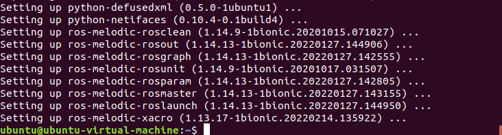
When you receive the following messages,the installation is successful.

Basic Syntax of URDF Model

1. XML Basic Syntax

The URDF model is written using XML standard.

Elements:

An element can be defined as desired using the following formula:

<element>

</element>

Properties:

Properties are included within elements to define characteristics and parameters. Please refer to the following formula to define an element with properties:

<element

property_1=”property value1”

property_2=”property value2”>

</element>

Comments:

Comments have no impact on the definition of other properties and elements. Please use the following formula to define a comment:

<!– comment content –>

2. Link

The Link element describes the visual and physical properties of the robot’s rigid component. The following tags are commonly used to define the motion of a link:

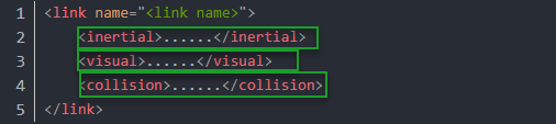
<visual>: Describe the appearance of the link, such as size, color and shape.

<inertial>: Describe the inertia parameters of the link, which will used in dynamics calculation.

<collision>: Describe the collision inertia property of the link

Each tag contains the corresponding child tag. The functions of the tags are listed below.

Tag	Function
origin	Describe the pose of the link. It contains two parameters, including xyz and rpy. Xyz describes the pose of the link in the simulated map. Rpy describes the pose of the link in the simulated map.
mess	Describe the mess of the link
inertia	Describe the inertia of the link. As the inertia matrix is symmetrical, these six parameters need to be input, ixx, ixy, ixz, iyy, iyz and izz, as properties. These parameters can be calculated.
geometry	Describe the shape of the link. It uses mesh parameter to load texture file, and em[ploys filename parameters to load the path for texture file. It has three child tags, namely box, cylinder and sphere.
material	Describe the material of the link. The parameter name is the required filed. The tag color can be used to change the color and transparency of the link.

3. Joint

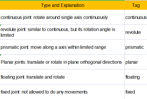
The “Joint” tag describes the kinematic and dynamic properties of the robot’s joints, including the joint’s range of motion, target positions, and speed limitations. In terms of motion style, joints can be categorized into six types.

The following tags will be used to write joint motion.

<parent_link>: Parent link

<child_link>: Child link

<calibration>: Calibrate the joint angle

<dynamics>: Describes some physical properties of motion

<limit>: Describes some limitations of the motion

The function of each tag is listed below. Each tag involves one or several child tags.

Tag	Function
origin	Describe the pose of the parent link. It involves two parameters, including xyz and rpy. Both xyz and rpy describe the pose of the link in simulated map.
axis	Control the child link to rotate around any axis of the parent link.
limit	The motion of the child link is constrained using the lower and upper properties, which define the limits of rotation for the child link. The effort properties restrict the allowable force range applied during rotation (values: positive and negative; units: N). The velocity properties confine the rotational speed, measured in meters per second (m/s).
mimic	Describe the relationship between joints.
safety_controller	Describes the parameters of the safety controller used for protecting the joint motion of the robot.

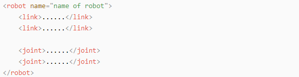
4. Robot Tag

The complete top tags of a robot, including the <link> and <joint> tags, must be enclosed within the <robot> tag. The format is as follows:

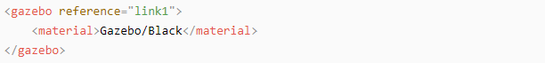
5. gazebo Tag

This tag is used in conjunction with the Gazebo simulator. Within this tag, you can define simulation parameters and import Gazebo plugins, as well as specify Gazebo’s physical properties, and more.

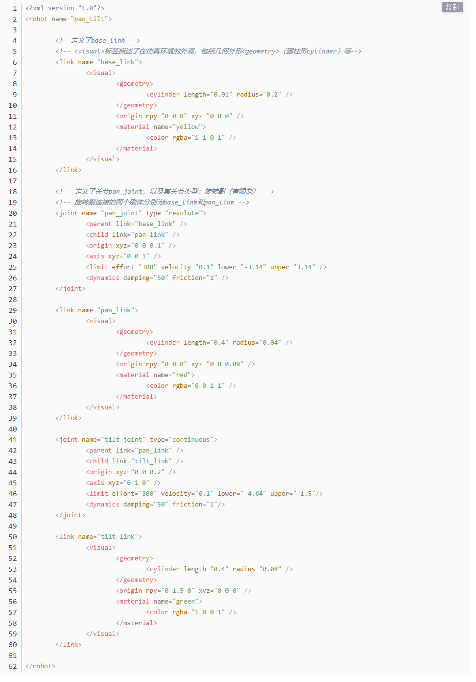
6. Write Simple URDF Model

Name the model of the robot

To start writing the URDF model, we need to set the name of the robot following this format: “<robot name=“robot model name”>”. Lastly, input “</robot>” at the end to represent that the model is written successfully.

Set links

To write the first link and use indentation to indicate that it is part of the currently set model. Set the name of the link using the following format: <link name=”link name”>. Finally, conclude with “</link>” to indicate the successful completion of the link definition.
Write the link description and use indentation to indicate that it is part of the currently set link, and conclude with <visual>.
The “<geometry>” tag is employed to define the shape of a link. Once the description is complete, include “</geometry>”. Within the “<geometry>” tag, indentation is used to specify the detailed description of the link’s shape. The following example demonstrates a link with a cylindrical shape: “<cylinder length=”0.01” radius=”0.2”/>”. In this instance, “length=”0.01”” signifies a length of 0.01 meters for the link, while “radius=”0.2”” denotes a radius of 0.2 meters, resulting in a cylindrical shape.
The “<origin>” tag is utilized to specify the position of a link, with indentation used to indicate the detailed description of the link’s position. The following example demonstrates the position of a link: “<origin rpy=”0 0 0” xyz=”0 0 0” />”. In this example, “rpy” represents the roll, pitch, and yaw angles of the link, while “xyz” represents the coordinates of the link’s position. This particular example indicates that the link is positioned at the origin of the coordinate system.
The “<material>” tag is used to define the visual appearance of a link, with indentation used to specify the detailed description of the link’s color. To start describing the color, include “<material>”, and end with “</material>” when the description is complete. The following example demonstrates setting a link color to yellow: “<color rgba=”1 1 0 1” />”. In this example, “rgba=”1 1 0 1”” represents the color threshold for achieving a yellow color.

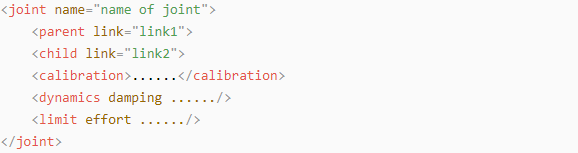
7. Set joint

To write the first joint, use indentation to indicate that the joint belongs to the current model being set. Then, specify the name and type of the joint as follows: “<joint name=”joint name” type=”joint type”>”. Finally, include “</joint>” to indicate the completion of the joint definition.

Note

Note: to learn about the type of the joint, please refer to joint.

Write the description section for the connection between the link and the joint. Use indentation to indicate that it is part of the currently defined joint. The parent parameter and child parameter should be set using the following format: “<parent link=”parent link”/>”, and “<child link=”child link” />”. With the parent link serving as the pivot, the joint rotates the child link.
“<origin>” describes the position of the joint using indention. This example describes the position of the joint: “<origin xyz=“0 0 0.1” />”. xyz is the coordinate of the joint.
“<axis>” describes the position of the joint adopting indention. “<axis xyz=“0 0 1” />” describes one posture of a joint. xyz specifies the pose of the joint.
“<limit>” imposes restrictions on the joint using indention. The below picture The “<limit>” tag is used to restrict the motion of a joint, with indentation indicating the specific description of the joint angle limitations. The following example describes a joint with a maximum force limit of 300 Newtons, an upper limit of 3.14 radians, and a lower limit of -3.14 radians. The settings are defined as follows: “effort=“joint force (N)”, velocity=“joint motion speed”, lower=“lower limit in radians”, upper=“upper limit in radians”.
“<dynamics>” describes the dynamics of the joint using indention. “<dynamics damping=“50” friction=“1” />” describes dynamics parameters of a joint.

The complete codes are as below.

12.1.2 ROS Robot URDF Model Description

Preparation

To grasp the URDF model, check out “12.1.1 URDF Model ->Basic Syntax of URDF Model” for the key syntax. This part quickly breaks down the robot model code and its components.

Check Code of Robot Model

Start the robot, and access the robot system desktop using NoMachine.
Click-on to open the command-line terminal.
Run the command ‘roscd hiwonder_description/urdf/’ to navigate to the directory containing programs.
```
roscd hiwonder_description/urdf/
```
Execute the command ‘vim jetrover.xacro’ to access the robot simulation model file.
```
vim jetrover.xacro
```
Locate the code below:

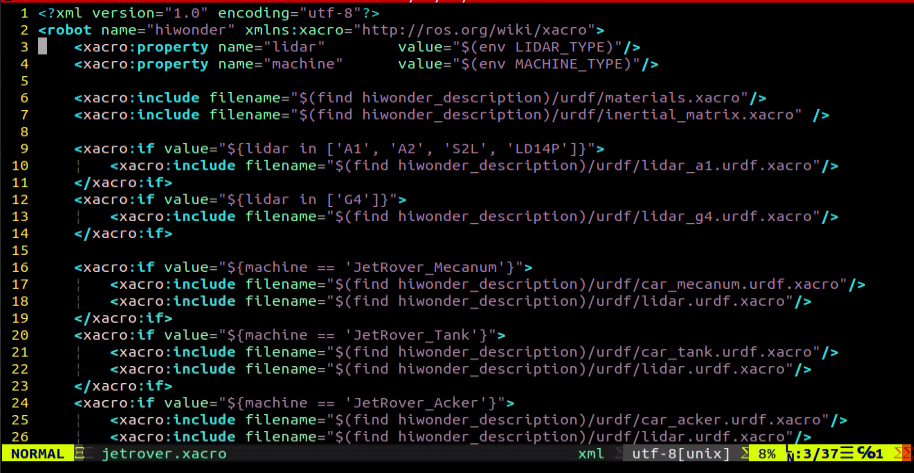
Several URDF models are combined to create a full robot:

File Name	Device
materials	Color
inertial_matrix	Inertia matrix
lidar_a1	A1 Lidar
lidar_g4	G4 Lidar
car_mecanum	Mecanum-wheel chassis
car_tank	Track chassis
car_acker	Ackermann chassis
Imu	Inertial measurement unit
depth_camera	Depth camera
common	Shared or common components or attributes
connect	Connector, describing the physical connection relationships between various components of the robot
arm	Robot arm
gripper	Gripper
arm.transmission	Transmission structure of the robotic arm
gripper.transmission	Transmission structure of the gripper

Brief Analysis of Robot’s Main Body Model

JetRover has three types of chassis: wheel, track, and Ackerman chassis. Here, we’ll focus on the Ackerman chassis as an example. Although the main model files for the wheel and track chassis are mostly the same, any differences will be explained later in this article.

To begin, open a new command terminal and type “vim car_acker.urdf.xacro” to access the robot model file, which contains the description of each part of the robot model.

vim car_acker.urdf.xacro

<?xml version="1.0" encoding="utf-8"?><robot name="hiwonder" xmlns:xacro="http://ros.org/wiki/xacro">

This is the beginning of the URDF file. It specifies the XML version and encoding, and defines a robot model named “hiwonder”. The xmlns:xacro namespace is utilized here to generate URDF using Xacro macro definitions.

The following line of code defines a Xacro property named “M_PI” and assigns the value of π to it.

 <xacro:property name="M_PI" value="3.1415926535897931"/>

In this section, a link named “base_footprint” is defined as the robot’s chassis.

 <link name="base_footprint"/>

Various characteristics of the robot such as mass, width, height, and depth are specified.

  <xacro:property name="base_link_mass"     value="1.6" /> 
  <xacro:property name="base_link_w"        value="0.30"/>
  <xacro:property name="base_link_h"        value="0.15"/>
  <xacro:property name="base_link_d"        value="0.10"/>

Next, a joint called base_joint is defined with a type of “fixed”, indicating it’s a stationary joint. It connects the parent link base_footprint with the child link base_link.

The joint’s position (origin) is determined using an xyz attribute, where ${0.05 + 0.0654867643253843} represents a calculated result.

Following this, a link named w_link is defined to represent a link component.

Lastly, a joint named w_joint is defined with type “fixed”, also being a stationary joint. It connects base_link as the parent link and w_link as the child link. Default values are used for the joint’s origin and axis.

<joint name="base_joint" type="fixed">
    <parent link="base_footprint"/>
    <child link="base_link"/>
    <origin xyz="0.0 0.0 ${0.05 + 0.0654867643253843}" rpy="0 0 0"/>
  </joint>
  <link name="w_link"/>
  <joint
    name="w_joint"
    type="fixed">
    <origin
      xyz="0 0 0"
      rpy="0 0 0" />
    <parent
      link="base_link" />
    <child
      link="w_link" />
    <axis
      xyz="0 0 0" />
  </joint>

This XML code defines a link within a robot model. Let’s dissect it to understand its structure and purpose.

The code begins with the <link> tag, naming the link base_green_link. Inside this tag, there are three main sections: <inertial>, <visual>, and <collision>.

The <inertial> section specifies the link’s inertial properties, like mass and inertia. It includes the <origin> tag, indicating the position and orientation of the inertial coordinate system relative to the link’s coordinate system. The <mass> tag denotes the link’s mass, and the <inertia> tag defines its moment of inertia about its principal axis.

The <visual> section determines the visual representation of the link. It includes the <origin> tag for the visualization coordinate system’s position and orientation relative to the link. The <geometry> tag defines the visual shape, here a grid, while the <mesh> tag specifies the file name of the mesh representing the link’s visual appearance. Lastly, the <material> tag specifies the color or texture, such as “green”.

The <collision> section specifies the link’s collision properties. It resembles the <visual> section but is for collision detection, not visualization. It includes the <origin> and <geometry> tags for defining position, direction, and shape of the collision representation.

In summary, this code defines a link in the robot model, detailing its inertial, visual, and collision properties. In simulations or visualizations, the mesh files specified in the <visual> and <collision> sections are utilized for visual representation and collision detection with other links.

 <link
    name="base_link">
    <xacro:box_inertial m="${base_link_mass}" w="${base_link_w}" h="${base_link_h}" d="${base_link_d}" x="0" y="0" z="-0.15" />
    <visual>
      <origin
        xyz="0 0 0"
        rpy="0 0 0" />
      <geometry>
        <mesh
          filename="package://hiwonder_description/meshes/acker/base_link.stl" />
      </geometry>
      <material name="black"/>
    </visual>
    <collision>
      <origin
        xyz="0 0 0"
        rpy="0 0 0" />
      <geometry>
        <mesh
          filename="package://hiwonder_description/meshes/acker/base_link.stl" />
      </geometry>
    </collision>
  </link>

This code defines a joint called base_green_joint, which is of type “fixed”, indicating it’s stationary. It connects the parent link base_link to the child link base_green_link. The joint’s coordinate origin is at (0, 0, 0), with Euler angles (rpy) set to (0, 0, 0), and no specific axis is defined for the joint.

<joint
    name="base_green_joint"
    type="fixed">
    <origin
      xyz="0 0 0"
      rpy="0 0 0" />
    <parent
      link="base_link" />
    <child
      link="base_green_link" />
    <axis
      xyz="0 0 0" />
  </joint>

Next, let’s examine the link description:

 <link
    name="wheel_left_front_link">
    <inertial>
      <origin
        xyz="-0.213334280297957 -0.203369638948946 -0.000334615151787748"
        rpy="0 0 0" />
      <mass
        value="0.124188560741815" />
      <inertia
        ixx="0.000108426797272382"
        ixy="4.75710998528631E-10"
        ixz="-4.51221408656634E-09"
        iyy="0.000198989755900859"
        iyz="1.62770134465076E-11"
        izz="0.000108425820065752" />
    </inertial>
    <visual>
      <origin
        xyz="0 0 0"
        rpy="0 0 0" />
      <geometry>
        <mesh
          filename="package://hiwonder_description/meshes/acker/wheel_left_front_link.stl" />
      </geometry>
      <material name="black"/>
    </visual>
    <collision>
      <origin
        xyz="0 0 0"
        rpy="0 0 0" />
      <geometry>
        <mesh
          filename="package://hiwonder_description/meshes/acker/wheel_left_front_link.stl" />
      </geometry>
    </collision>
  </link>

The provided code describes a link named wheel_left_front_link. This link includes inertial, visual, and collision information.

Inertial properties specify the link’s mass and inertial matrix. The mass is 0.124188560741815, and specific values are assigned to each component of the inertia matrix.

Visual properties define the link’s appearance using a three-dimensional model (mesh) with the file name “package://hiwonder_description/meshes/acker/wheel_left_front_link.stl”. Additionally, the link is colored with a material named “black”.

Collision properties determine the link’s collision shape, also utilizing a 3D model with the same file name as the visual representation.

<joint
    name="wheel_left_back_joint"
    type="fixed">
    <origin
      xyz="0.106753653016542 -0.0920004072996187 -0.0658214520621466"
      rpy="0 0 3.14158803228829" />
    <parent
      link="base_link" />
    <child
      link="wheel_left_back_link" />
    <axis
      xyz="0 0 0" />
  </joint>

The following XML code defines a joint and a link within a robot model.

Joint Definition:

Name: “wheel_left_back_joint”
Type: “fixed” (indicating a fixed joint)
Origin: Specifies the joint’s position and orientation relative to the parent link (“base_link”).
Parent Link: Specifies the parent link of the joint.
Sublink: Specifies the sublink of the joint.
Axis: Specifies the axis of rotation of the joint. Here, it’s set to (0, 0, 0), indicating it’s a fixed joint and doesn’t rotate.

Link Definition:

Name: “wheel_left_back_link”
Inertia: Specifies inertial properties of the link (mass, center of mass, and inertia).
Visualization: Specifies a visual representation of the link, including its position, orientation, geometry (grid), and material.
Collision: Specifies the link’s collision properties, including its position, orientation, and geometry (mesh).

 <joint
    name="wheel_left_back_joint"
    type="fixed">
    <origin
      xyz="0.106753653016542 -0.0920004072996187 -0.0658214520621466"
      rpy="0 0 3.14158803228829" />
    <parent
      link="base_link" />
    <child
      link="wheel_left_back_link" />
    <axis
      xyz="0 0 0" />
  </joint>

Link Definition:

Name: “wheel_right_front_link”
Inertia: Specifies the link’s inertial properties, including mass and inertia matrix.
Visualization: Defines the link’s visual appearance, including its position, orientation, geometry (mesh), and material.
Collision: Describes the link’s collision properties, including its position, orientation, and geometry (mesh).

Specifically:

Inertial: Specifies the mass and inertia matrix of the link. In this example, the link has a mass of 0.124186629923608, and specific values are assigned to individual components of the inertia matrix (ixx, ixy, ixz, iyy, iyz, izz).
Visual: Specifies the visual representation of the link. It utilizes a mesh file located at “package://hiwonder_description/meshes/acker/wheel_right_front_link.stl”, and the material used for visualization is called “black”.
Collision: Defines the collision properties of the link, which are identical to its visual properties and utilize the same mesh file.

<link
    name="wheel_right_front_link">
    <inertial>
      <origin
        xyz="-0.213332807255404 0.203675464611681 -0.000332210127461456"
        rpy="0 0 0" />
      <mass
        value="0.124186629923608" />
      <inertia
        ixx="0.000108439206695888"
        ixy="6.85847929033569E-10"
        ixz="-1.92360226002088E-08"
        iyy="0.00019900428610234"
        iyz="-1.53831301269727E-09"
        izz="0.00010842875904821" />
    </inertial>
    <visual>
      <origin
        xyz="0 0 0"
        rpy="0 0 0" />
      <geometry>
        <mesh
          filename="package://hiwonder_description/meshes/acker/wheel_right_front_link.stl" />
      </geometry>
      <material name="black"/>
    </visual>
    <collision>
      <origin
        xyz="0 0 0"
        rpy="0 0 0" />
      <geometry>
        <mesh
          filename="package://hiwonder_description/meshes/acker/wheel_right_front_link.stl" />
      </geometry>
    </collision>
  </link>

The code below describes a fixed joint connecting two links named base_link and wheel_right_front_link. The initial position and rotation of the joint are specified by the <origin> tag.

Attributes:

name=”wheel_right_front_joint”: Specifies the joint’s name as “wheel_right_front_joint”.
type=”fixed”: Indicates the joint type as “fixed”, meaning it’s stationary and cannot move.
<origin> tag: Defines the initial position and rotation of the joint. It sets the joint’s xyz coordinates as “-0.10658 0.091851 -0.065487” and the rpy rotation angles as “0 0 3.1416”.
<parent> tag: Specifies the parent link of the joint, which is “base_link”.
<child> tag: Specifies the child link of the joint, which is “wheel_right_front_link”.
<axis> tag: Defines the joint axis. In this case, it’s set to (0, 0, 0), indicating no specific axis is defined.

 <joint
    name="wheel_right_front_joint"
    type="fixed">
    <origin
      xyz="-0.10658 0.091851 -0.065487"
      rpy="0 0 3.1416" />
    <parent
      link="base_link" />
    <child
      link="wheel_right_front_link" />
    <axis
      xyz="0 0 0" />
  </joint>

The following describes a link named wheel_right_back_link, detailing its inertia properties, visualization properties, and collision properties. The geometry of the link utilizes a mesh file, and the visual properties specify a black material.

Attributes:

name=”wheel_right_back_link”: Specifies the link’s name as “wheel_right_back_link”.

Inertial Properties:
<inertial> tag: Defines the link’s inertial properties, including mass and inertia matrix.
<origin> tag: Specifies the position and rotation of the link’s inertial origin. Coordinates are set to “0.21333 0.20224 0.00032742”, with no rotation.
<mass> tag: Sets the link’s mass to “0.13231”.
<inertia> tag: Specifies the inertia matrix of the link.

Visualization Properties:
<visual> tag: Defines the link’s visual properties, including appearance and material.
<origin> tag: Specifies the position and rotation of the link’s visual origin. Coordinates are set to “0 0 0”, with no rotation.
<geometry> tag: Defines the link’s geometry, utilizing a mesh file.
<mesh> tag: Specifies the mesh file used for the link’s geometry, located at “package://hiwonder_description/meshes/acker/wheel_right_back_link.stl”.
<material> tag: Defines the material of the link as “black”.

Collision Properties:
<collision> tag: Defines the link’s collision properties, including geometry.
<origin> tag: Specifies the position and rotation of the link’s collision origin. Coordinates are set to “0 0 0”, with no rotation.
<geometry> tag: Defines the link’s collision geometry, using the same mesh file as the visual representation.

<link
    name="wheel_right_back_link">
    <inertial>
      <origin
        xyz="0.21333 0.20224 0.00032742"
        rpy="0 0 0" />
      <mass
        value="0.13231" />
      <inertia
        ixx="0.00010909"
        ixy="-8.0297E-09"
        ixz="1.1828E-08"
        iyy="0.00019967"
        iyz="-6.196E-09"
        izz="0.00010906" />
    </inertial>
    <visual>
      <origin
        xyz="0 0 0"
        rpy="0 0 0" />
      <geometry>
        <mesh
          filename="package://hiwonder_description/meshes/acker/wheel_right_back_link.stl" />
      </geometry>
      <material name="black"/>
    </visual>
    <collision>
      <origin
        xyz="0 0 0"
        rpy="0 0 0" />
      <geometry>
        <mesh
          filename="package://hiwonder_description/meshes/acker/wheel_right_back_link.stl" />
      </geometry>
    </collision>
  </link>

The following code still describes a joint. The name of this joint is “wheel_right_back_joint”.

Attributes:

name=”wheel_right_back_joint”: Specifies the joint’s name as “wheel_right_back_joint”.
type=”fixed”: Indicates that the joint type is “fixed”, meaning it’s a fixed joint that doesn’t allow movement.

Origin:
<origin>: Defines the origin position and posture of the joint.
xyz=”0.10675 0.091848 -0.065821”: Specifies the coordinates of the joint’s origin position in three-dimensional space as (0.10675, 0.091848, -0.065821).
rpy=”0 0 3.1416”: Represents the origin posture of the joint using Euler angles, where roll, pitch, and yaw are 0, 0, and 3.1416 respectively.
Parent and Child Links:
<parent>: Defines the parent link of the joint.
link=”base_link”: Specifies that the parent link of this joint is named “base_link”.
<child>: Defines the child link of the joint.
link=”wheel_right_back_link”: Specifies that the child link of this joint is named “wheel_right_back_link”.

Axis:
<axis>: Defines the axis of the joint.
xyz=”0 0 0”: Indicates that the axis of this joint is (0, 0, 0), meaning the axis is not specifically defined.
Closing Tag:
</joint>: Closes the joint element.

 <joint
    name="wheel_right_back_joint"
    type="fixed">
    <origin
      xyz="0.10675 0.091848 -0.065821"
      rpy="0 0 3.1416" />
    <parent
      link="base_link" />
    <child
      link="wheel_right_back_link" />
    <axis
      xyz="0 0 0" />
  </joint>

12.2 MoveIt Simulation V1.0

12.2.1 MoveIt Configuration

Note

Note: The MoveIt configuration has been pre-set before delivery, and there’s no need to modify it. This section simply provides an overview of the configuration. If you wish to directly experience the game, feel free to skip this step.

MoveIt Introduction

MoveIt is composed of manipulation function packs of ROS. By incorporating the latest advances in motion planning, manipulation, 3D perception, kinematics, collision detection, MoveIt is state of the art software for mobile manipulation.

It is a user-friendly platform used to develop advanced robot applications and assess new robot design. Besides, it is an open-source software widely applied in industrial, commercial, R&D and other fields.

In addition, MoveIt provides series of mature plugins and tools to achieve rapid robotic arm control configuration. Large amount of API are encapsulated facilitating your secondary development and creative application development.

Enable Configuration Program

Note

Note: the input command should be case sensitive and keywords can be complemented using Tab key.

Start the robot, and access the robot system desktop using the remote control software.
Click-on to open the command-line terminal.
Execute the command ‘sudo systemctl stop start_app_node.service’, and hit Enter to disable the app auto-start service.
```
sudo systemctl stop start_app_node.service
```
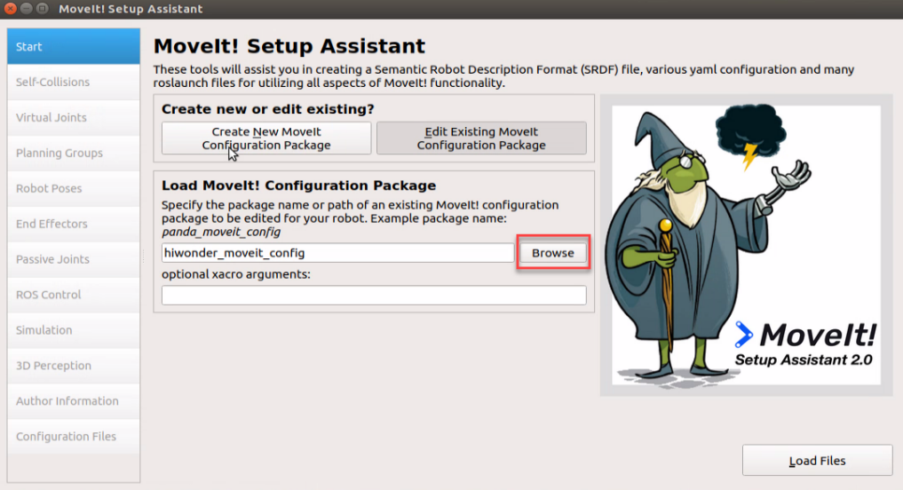
Run the command ‘roslaunch hiwonder_moveit_config setup_assistant.launch’ to start MoveIt assistant.
```
roslaunch hiwonder_moveit_config setup_assistant.launch
```
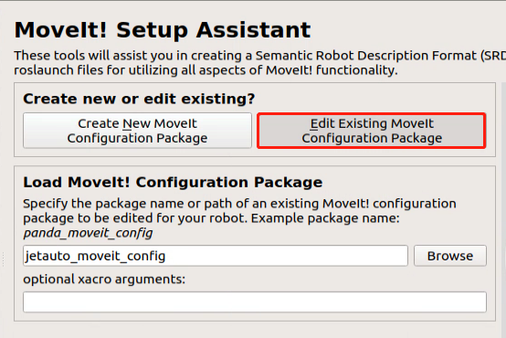
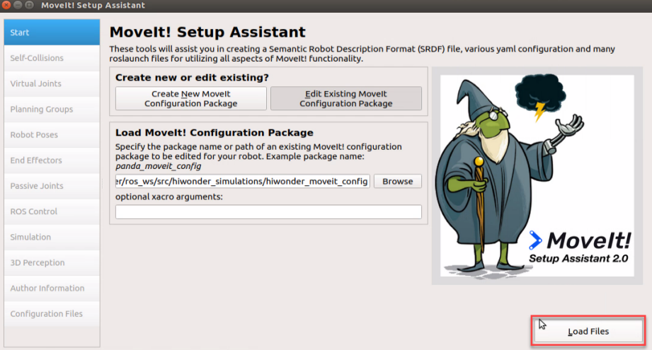
Click “Edit Existing MoveIt Configuration Package” to edit the existed configuration pack.
Click “Browse > home/home/ros_ws/src/hiwonder_simulations/hiwonder_moveit_config” as pictured.
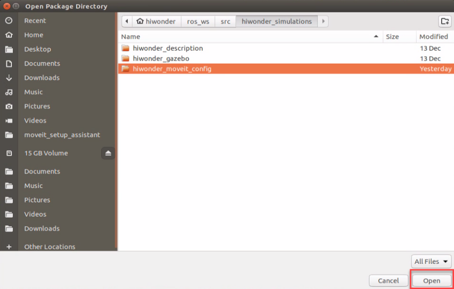
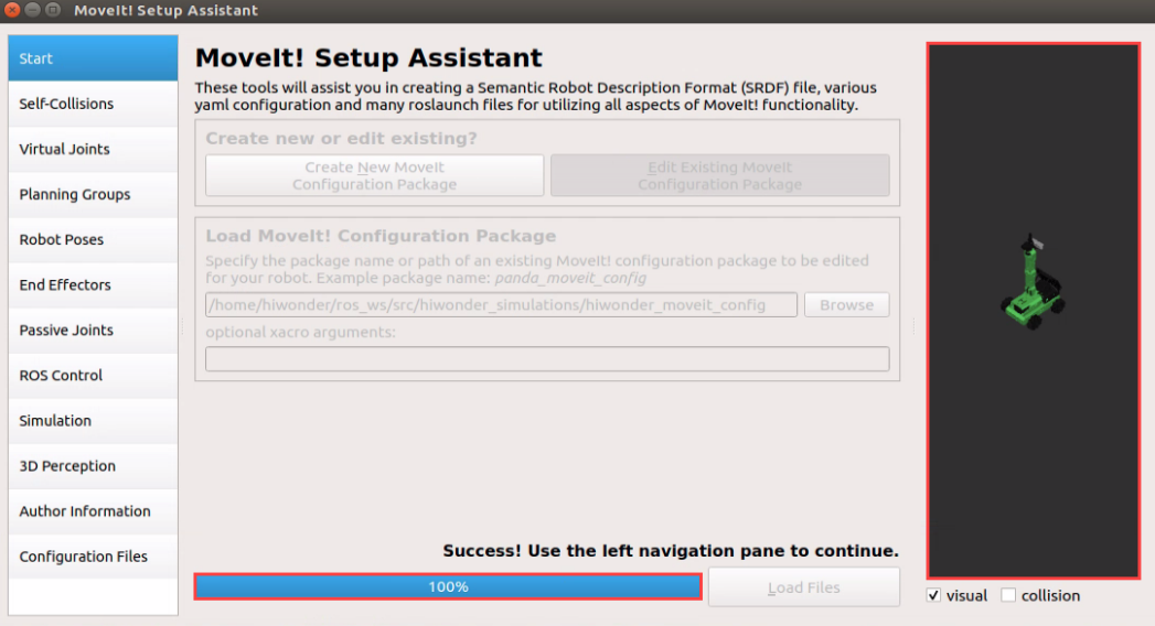
Click “Load Files” and wait for the file to finish loading.

When it is loaded to 100%, the robot model will appear, which means that the file is loaded successfully.
Configure the contents of “Virtual joints” and “Robot pose” at left side.

Note

Note: Reconfiguring will overwrite previous settings. If errors occur during the process, it may result in the functionality not working properly.

Configuration Introduction

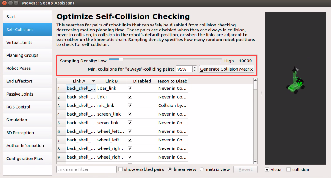
1. Self-Collisions

Generate a custom collision matrix. The default collision matrix generator scans all joints of the robot. This collision matrix can be safely disabled to reduce the processing time for motion planning.

Sampling density refers to how many random joints are extracted to check for collisions. Higher density requires more computation time, with the default value set at 10,000 collision checks.

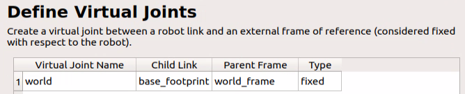
2. Virtual joints

Include virtual joints, primarily used for linking the robot to the simulation program. Here, we define a virtual joint to connect the base_footprint and world_frame frames.

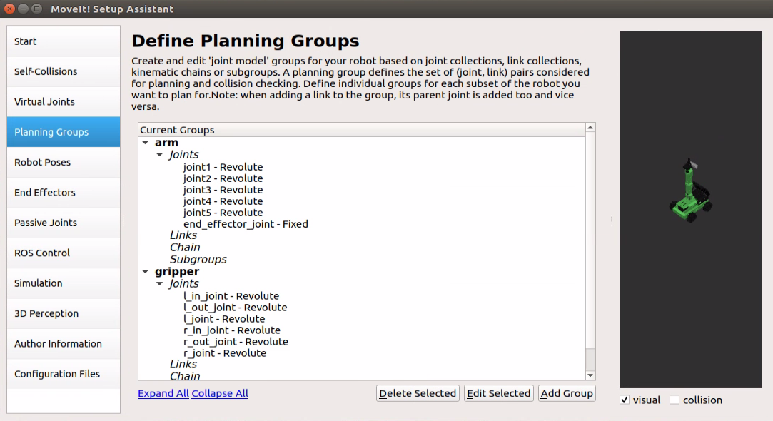
3. Planning Groups

Add joint combinations, primarily used to describe the various joint components required to compose the robot.

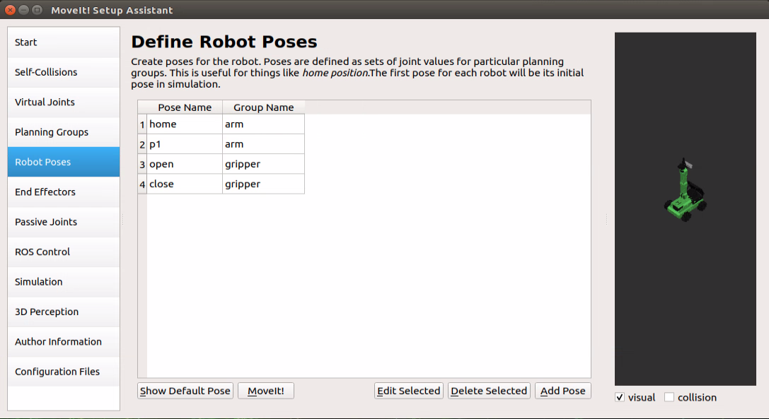
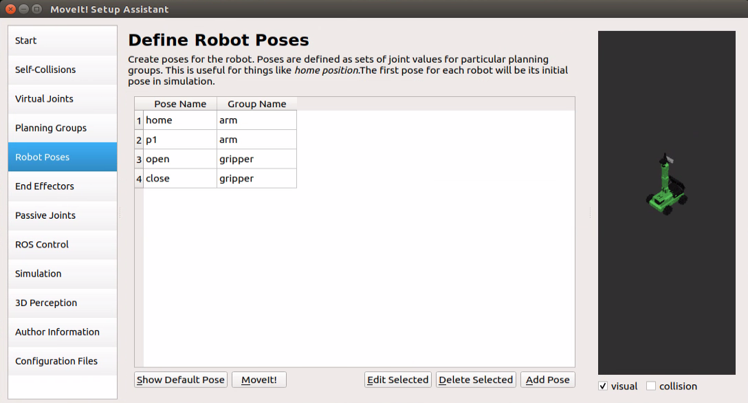
4. Robot Poses

Define the robot’s pose, pose name and the joints will be used to form this pose.

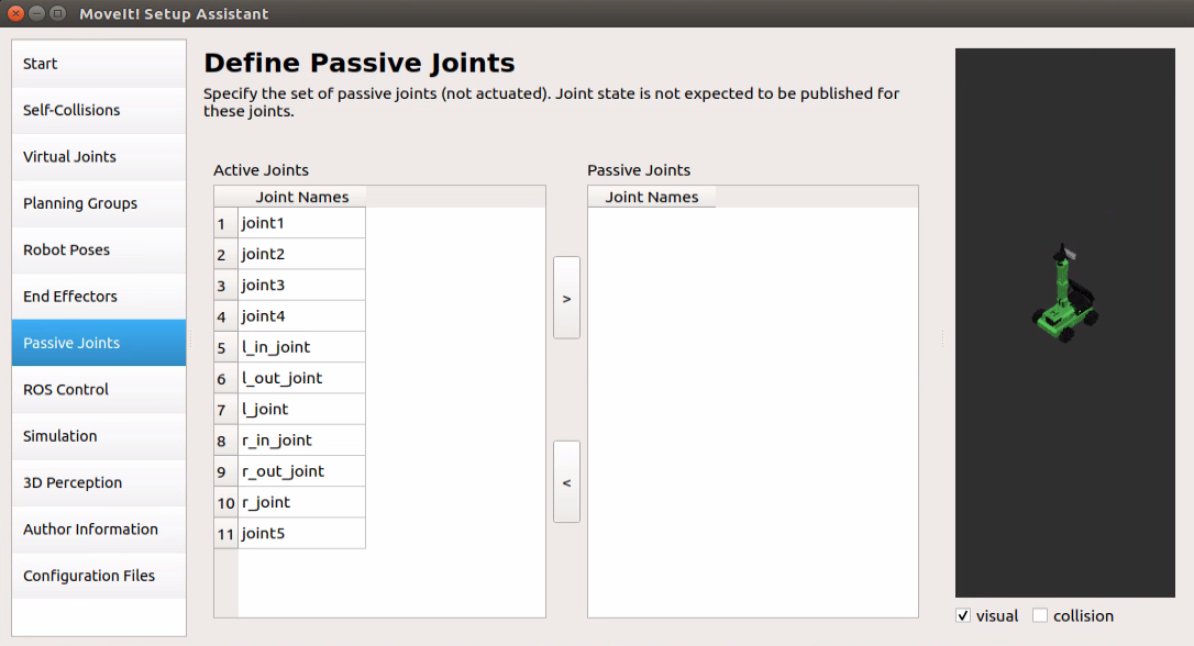
5. Passive Joints

Specify the joints that are excluded from use, those that are available for use, and those that are not permissible for use.

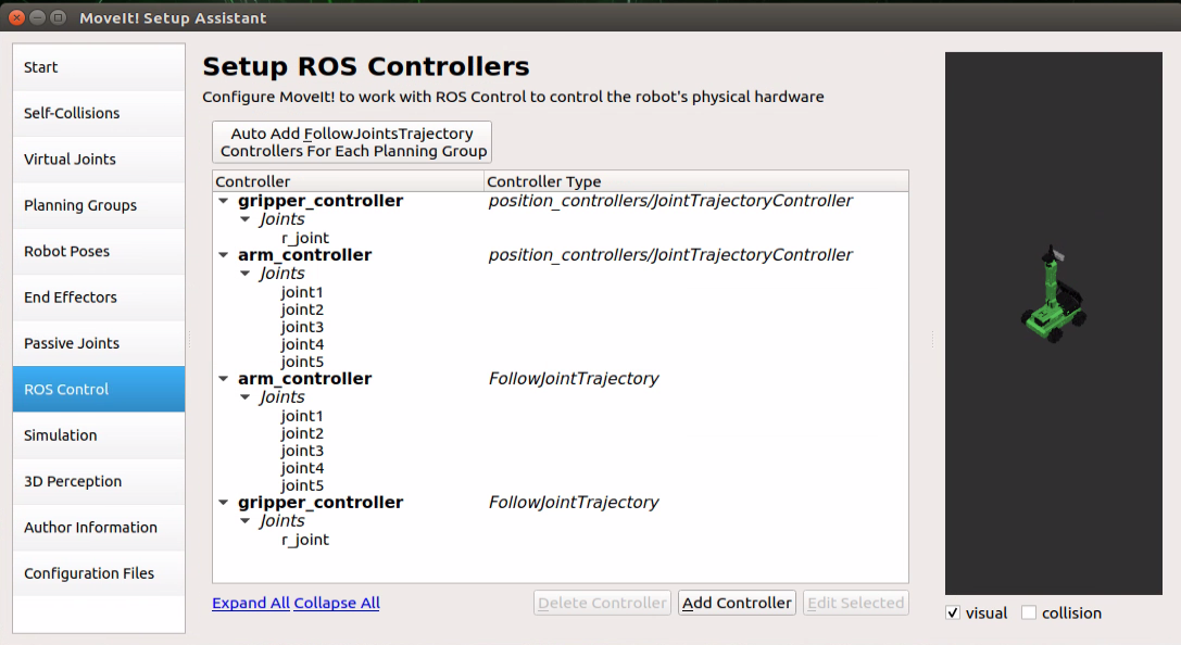
6. ROS Control

In this context, we can use the ROS Control panel to add a simulation controller to the joints, enabling the simulation of robotic arm movements through MoveIt.

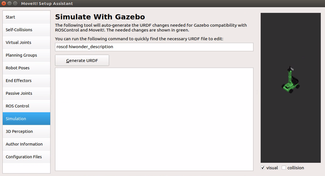
7. Simulation

Set up the Gazebo simulation and configure it by specifying the necessary URDF file for the simulation.

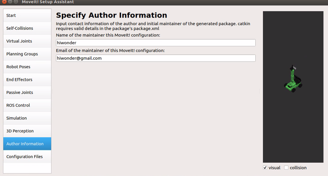
8. Author Information

Add author information.

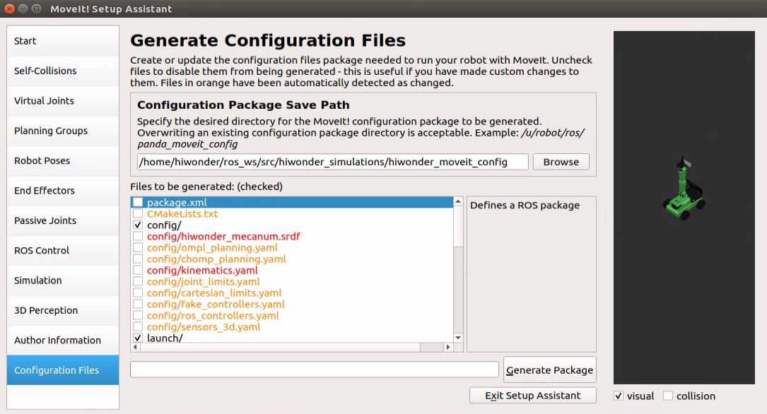
9. Configuration Files

Create configuration files and indicate the preferred directory for the generated configuration package. Subsequently, click on ‘Generate Package’ to generate the configuration package.

12.2.2 MoveIt Use Notice & Control

Use Notice

Before you begin, ensure there’s ample space around the robot. Maintain a safe distance during gameplay to prevent any collisions between the robot arm and surroundings, which could cause damage. Additionally, bend the antenna backward to prevent interference with the robot arm’s movement and avoid damaging the antenna.

In this section, MoveIt will be utilized to plan paths and control both the simulation model and the actual manipulator, guiding them to specific locations according to the planned path.

Enable Related Service

Note

Note: the input command should be case sensitive, and keywords can be complemented using Tab key.

Start the robot, and access the robot system desktop using NoMachine remote control software.
Click-on to open the command-line terminal.
Execute the command ‘sudo systemctl stop start_app_node.service’, and hit Enter to terminate the app auto-start service.
```
sudo systemctl stop start_app_node.service
```
Open a new terminal, and run the command ‘roslaunch hiwonder_moveit_config demo.launch fake_execution:=false’ to launch MoveIt tool.
```
roslaunch hiwonder_moveit_config demo.launch fake_execution:=false
```

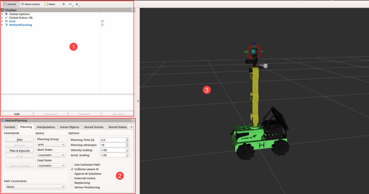
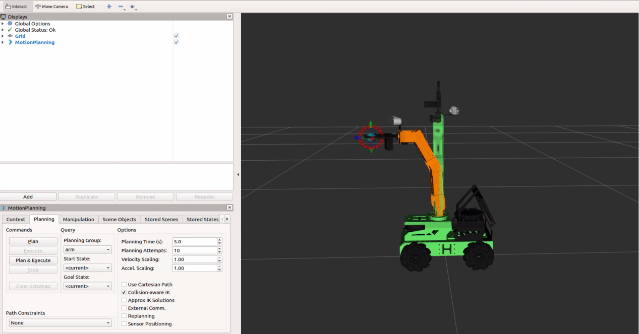
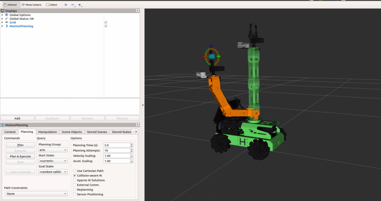
The software interface is as below:

: RVIZ tool bar;
: Movelt debugging area;
: Simulation model adjustment area

Control Instructions

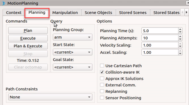
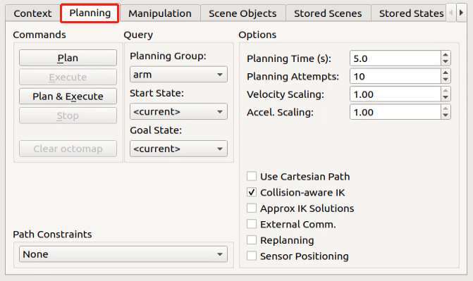
Navigate to the ‘Planning’ section in the MoveIt debugging area.
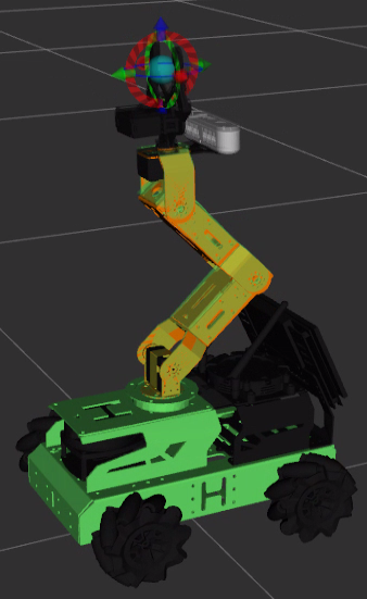
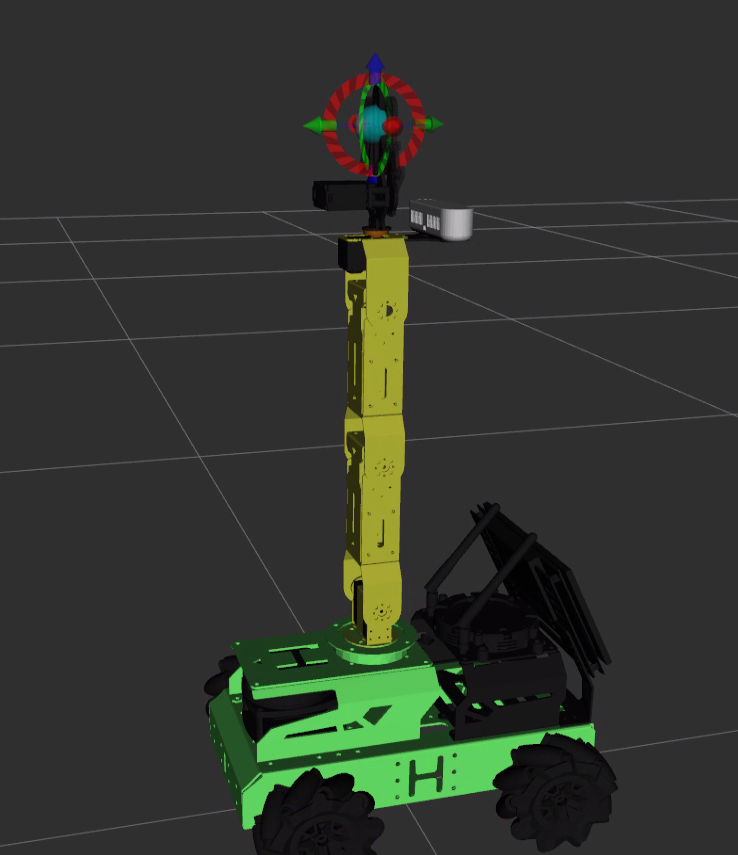
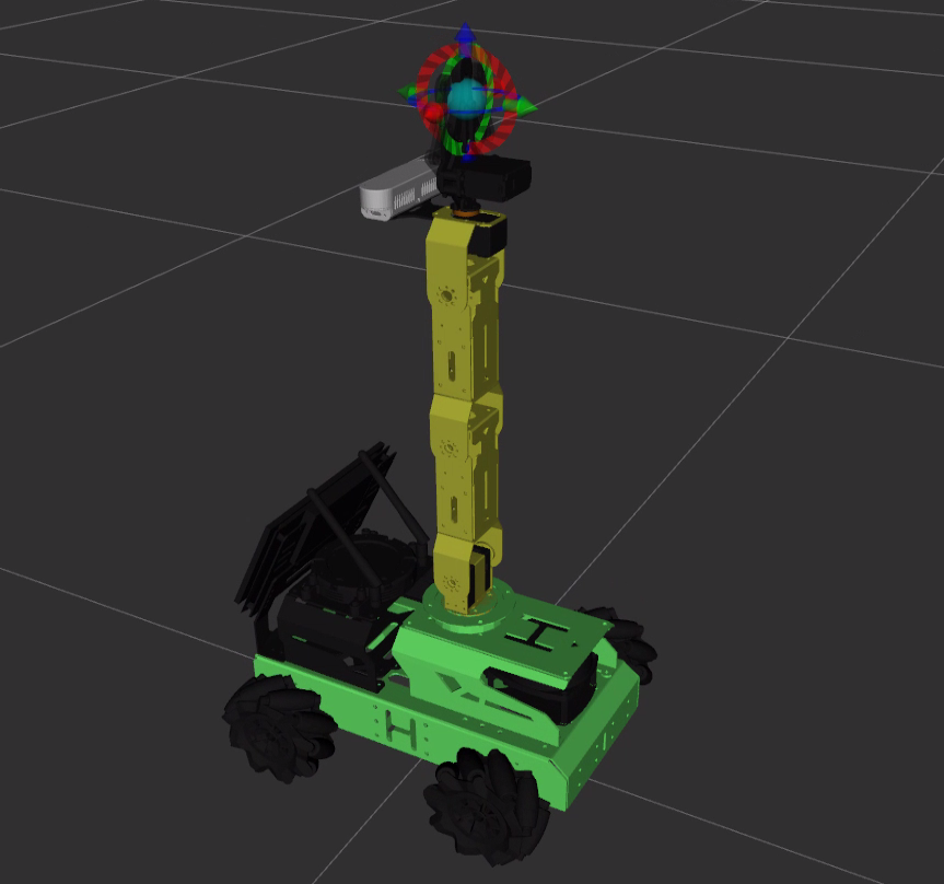
In the simulation model adjustment area, you’ll see red, green, and blue arrows. Click and drag these arrows to adjust the posture of the robotic arm. Imagine yourself facing the robot:

Green arrow corresponds to the X-axis direction, with the positive direction being to the left of the robot.
Red arrow corresponds to the Y-axis direction, with the positive direction being to the front of the robot.
Blue arrow corresponds to the Z-axis direction, with the positive direction being above the robot.

Besides using the arrows for overall adjustments, you can also fine-tune individual joints directly. Click the triangle icon on the right side, then locate and click on the “Joints” panel.
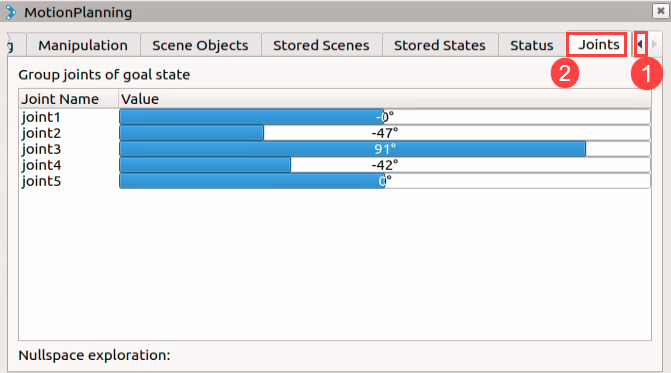
Drag the sliders to adjust the angle of the corresponding joint.
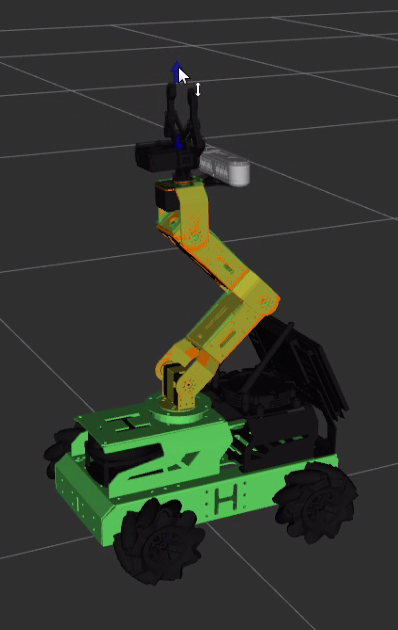
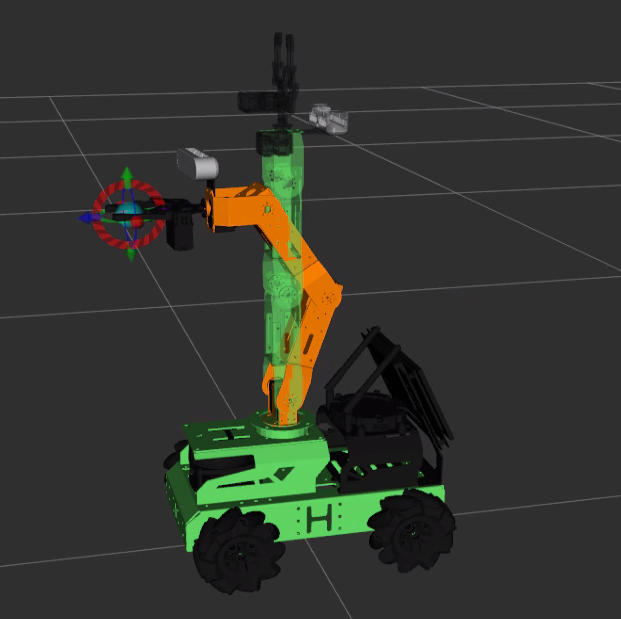
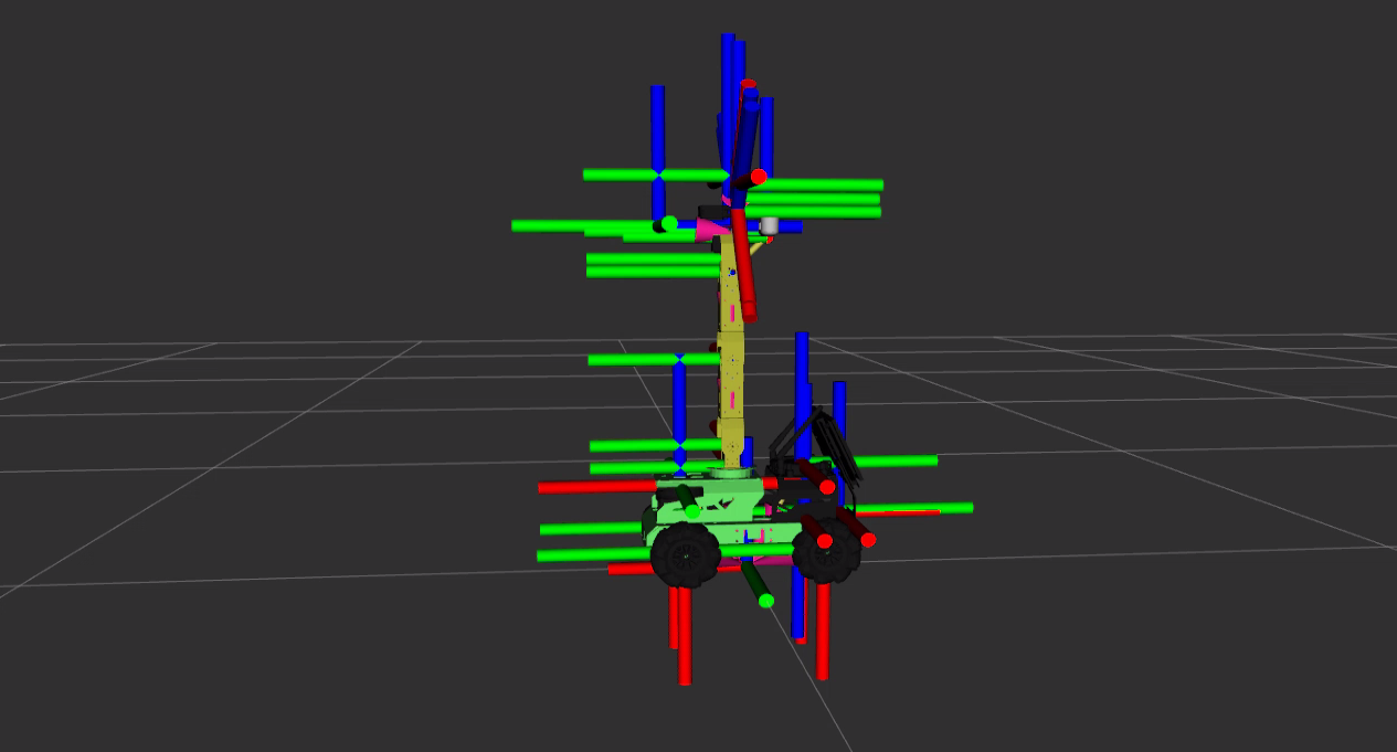
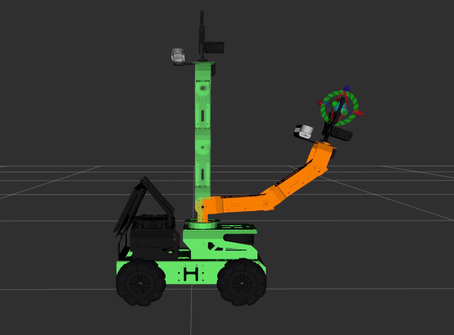
After planning the movement path of the robot arm, the new position will be indicated in orange if the path is clear. However, if the new position collides with other parts of the robot, it will be marked in red. In such cases, you need to readjust it to ensure there are no collisions before proceeding with the action execution.

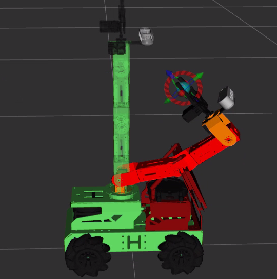
For instance, if the robot arm is positioned as depicted below, it would collide with our depth camera. Hence, it’s marked as a red state, indicating it cannot be executed, as shown:

After planning the path, navigate back to the “Planning” section and select the “Plan” option. This will display the movement path of the simulation model, illustrating the transition from the initial position to the newly planned position.
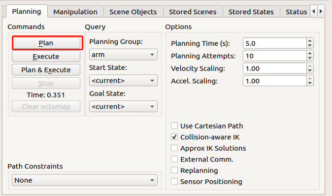
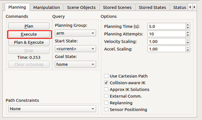
Finally, click on “Execute” to activate the planned motion for both the simulation model and the robotic arm.

Note

Note: During the initial execution, the robot arm will quickly return to a straight position before proceeding with the planned movement.

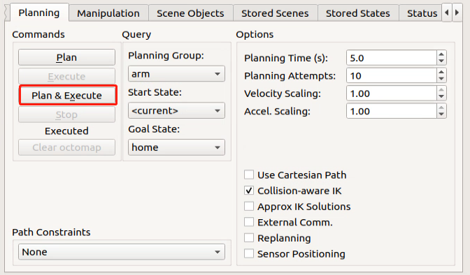
Click-on ‘Plan & Execute’, then the model will move along the newly planned path.

If you need to terminate this game, you can use short-cut ‘Ctrl+C’. If the game cannot be shutdown, please retry.

After finishing the game experience, you can activate the mobile app service either through commands or by restarting the robot. Without the mobile app service turned on, the app’s features won’t work. (Note: If the robot restarts, the mobile app service will start automatically.)

To restart the mobile app service, enter the command: “sudo systemctl restart start_app_node.service”. Then, wait for the robot arm to return to its initial posture and for the service startup to complete.

sudo systemctl restart start_app_node.service

12.2.3 MoveIt Random Motion

Notice

Before beginning, ensure there’s adequate space around the robot. Maintain a safe distance during gameplay to prevent collisions between the robot arm and surrounding objects, which could cause damage. Also, bend the antenna backward to prevent the robot arm from colliding with and damaging the antenna.

In this section, MoveIt will be utilized to plan paths and control both the simulation model and the actual manipulator, guiding them to random positions.

Enable Related Service

Note

Note: the input command should be case sensitive, and keywords can be complemented using Tab key.

Start the robot, and access the robot system desktop using NoMachine remote control software.
Click-on to open the command-line terminal.
Execute the command ‘sudo systemctl stop start_app_node.service’, and hit Enter to terminate the app auto-start service.
```
sudo systemctl stop start_app_node.service
```
Open a new command-line terminal, and run the command ‘roslaunch hiwonder_moveit_config demo.launch fake_execution:=false’ to launch MoveIt tool.
```
roslaunch hiwonder_moveit_config demo.launch fake_execution:=false
```

The software interface is as below:

: RVIZ tool bar;
: Movelt debugging area;
: Simulation model adjustment area

Random Motion

In the MoveIt debugging area, locate the “Planning” section.
In the simulation model adjustment area, you’ll see arrows in three colors: red, green, and blue. Imagine you’re facing the robot:

Green represents the X-axis direction, with the positive direction to the left of the robot.
Red indicates the Y-axis direction, with the positive direction in front of the robot.
Blue signifies the Z-axis direction, with the positive direction above the robot.

In the “Query” category, click on the drop-down menu labeled “Planning Group” and choose the joint group (also known as server group) you want to control. For instance, the default example here is the “arm” group.
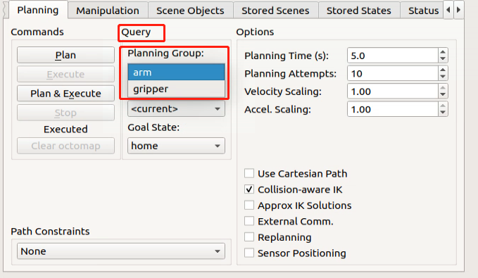
Select the desired goal position from the drop-down menu labeled ‘Goal State’.
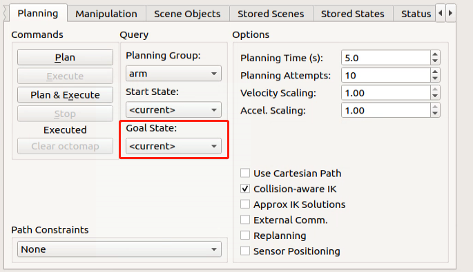
The drop-down menu is as below:

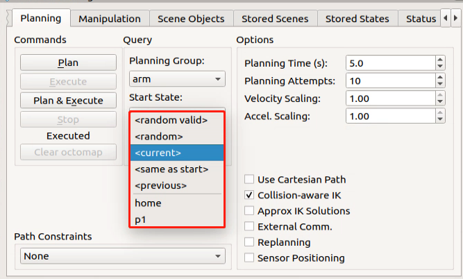
The parameters have the following meanings:

“random valid”: A randomly chosen position where there will be no collisions.

“random”: A randomly chosen position, which may result in a collision.

“current”: The current position.

“same as start”: Same as the starting position.

“previous”: The previous target position.

Additionally, the options “home” and “p1” are default locations set by the program.
To prevent random collisions, we choose “random valid” to generate a randomized target position. Each selection will create a new target position without any risk of collision, which will be displayed alongside the simulation model.
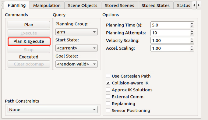
Click “Plan & Execute”, and both the simulation model and the robotic arm will move simultaneously. The simulation model will demonstrate the newly planned movement path, while the robotic arm executes the action.

Note

Note: it is normal that the model reacts slowly after you click-on ‘Plan’ icon!

If you need to terminate this game, you can use short-cut ‘Ctrl+C’. If the game cannot be shutdown, please retry.

Execute the command ‘sudo systemctl restart start_app_node.service’ to restart the service. If you need to input the password, you need to enter the password ‘hiwonder’.

sudo systemctl restart start_app_node.service

12.2.4 MoveIt Kinematics Design

Kinematics Introduction

Kinematics, as a branch of mechanics focused on geometric aspects (excluding the physical properties of objects and forces applied to them), explores and describes the principles governing changes in the position of objects over time. In the context of robotics, two distinct methods—forward kinematics and inverse kinematics—address the dynamics of motion.

Forward kinematics entails determining the position and orientation of the end effector based on the values of joint variables. In simpler terms, it calculates the final position and orientation of the robot by considering the angles of rotation of its servos.

Conversely, inverse kinematics involves determining the values of robot joint variables given the position and orientation of the end effector. It requires calculating the angles of rotation that the servos must achieve based on the final position and orientation of the robot.

Forward Kinematics Analysis

1. DH Parameter Introduction

Denavit-Hartenberg (DH) parameters form a mathematical model used to describe the spatial relationships and coordinate system determination between two pairs of joint linkages in a robotic system. The four DH parameters chosen each possess clearly defined physical meanings, as elaborated below:

link length : The length of the common normal between the axes of the two joints (Rotation axis of rotation joint, translation axis of translation joint)
link twist: The angle at which the axis of one joint rotates around their common normal relative to the axis of the other joint
link offset: The common normal of one joint and the next joint and the distance between the common normal of one joint and the previous joint along this joint axis
joint angle: The common normal of one joint and the next joint and the angle of rotation around the joint axis with the common normal of the previous joint

The above definition is very complicated, but it will be much clearer when combined with the coordinate system.

First of all you should pay attention to the two most important “lines”: the joint axis, and the common normal between the axis joint and the adjacent joint.

In the DH parameter system, we set axis as the z axis; common normal as the x axis, and the direction of the x axis is: from this joint to the next joint.

Of course, these two rules alone are not enough to completely determine the coordinate system of each joint. Let’s talk about the steps to determine the coordinate system in detail below.

In applications such as the simulation of the robotic arm, we often adopt other methods to establish the coordinate system, but mastering the methods mentioned here is necessary for you to understand the mathematical expression of the robotic arm and understand our subsequent analysis.

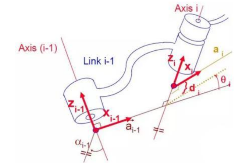
The figure below shows two typical robot joints. Although such joints and links are not necessarily similar to the joints and links of any actual robot, they are very common and can easily represent any joint of the actual robot.

2. Determine the Coordinate System

To determine the coordinate system, there are generally the following steps:

In order to model the robot with DH notation, the first thing is to specify a local ground reference coordinate system for each joint, so a Z axis and an X axis must be specified for each joint.

Specify the Z axis. If the joint is rotating, the Z axis is in the direction of rotation according to the right-hand rule. The rotation angle around the Z axis is a variable of the joint; if the joint is a sliding joint, the Z axis is the direction of movement along a straight line. The link length d along the Z axis is the joint variable.

Specify the X axis.When the two joints are not parallel or intersect, the Z axis is usually a diagonal line, but there is always a common vertical line with the shortest distance, which is orthogonal to any two diagonal lines. Define the X axis of the local reference coordinate system in the direction of the common perpendicular. If an represents the common perpendicular between Zn1, the direction of Xn will be along an.

Of course there are special circumstances. When the Z axes of the two joints are parallel, there will be countless common perpendiculars. At this time, you can select the one that is collinear with the common perpendicular of the previous joint, which can simplify the model; if two joints intersect, there is no common perpendicular between them. In this case, the line perpendicular to the plane formed by the two axes can be defined as X Shaft can simplify the model.

After attaching the corresponding coordinate system to each joint, as shown in the following figure:

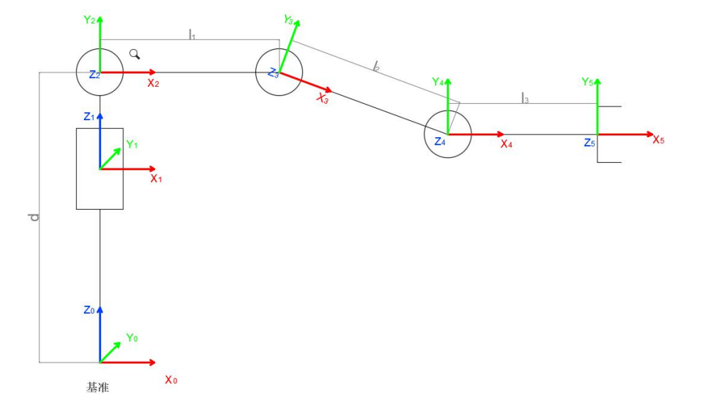
After determining the coordinate system, we can express the above four parameters in a more concise way:

link length i 1: the distance from Zi 1 to Zi along Xi 1

link twist i 1 : Zi the angle of Zi relative to Zi 1 to rotate around Xi 1

link offset i d :the distance from Xi 1 to Xi 1 along Zi

joint angle i : Xi relative to Xi 1 around Zi

12.2.5 Inverse Kinematic Analysis

For the robot arm, the position and orientation of the gripper are given to obtain the rotation angle of each joint. The three-dimensional motion of the robotic arm is more complicated. In order to simplify the model, we remove the rotation joint of the station so that the kinematics analysis can be performed on a two-dimensional plane.

Inverse kinematics analysis generally requires a large number of matrix operations, and the process is complex and computationally expensive, so it is difficult to implement. In order to better meet our needs, we use geometric methods to analyze the robotic arm.

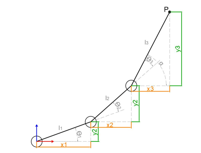
We simplify the model of the robotic arm, remove the base pan/tilt, and the actuator part to get the main body of the robotic arm. From the figure above, you can see the coordinates (x, y) of the end point P of the robotic arm, which ultimately consists of three parts (x1+x2+x3, y1+y2+y3).

Among them θ1, θ2,θ3 in the above figure are the angles of the servo that we need to solve, and α is the angle between the paw and the horizontal plane. From the figure, it is obvious that the top angle of the claw α=θ1+θ2+θ3, based on which we can formulate the following formula:

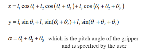
Among them, x and y are given by the user, and l1, l2, and l3 are the inherent properties of the mechanical structure of the robotic arm.

In order to facilitate the calculation, we will deal with the known part and consider the whole:

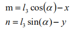
Substituting m and n into the existing equation, and then simplifying can get:

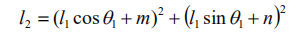
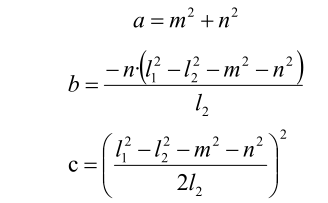
Through calculation:

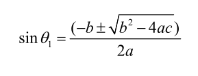
We see that the above formula is the root-finding formula of a quadratic equation in one variable:

Based on this, we can find the angle of θ1, and similarly we can also find θ2. From this we can obtain the angles of the three steering gears, and then control the steering gears according to the angles to realize the control of the coordinate position.

12.2.6 Robot Arm Coordinate System Introduction

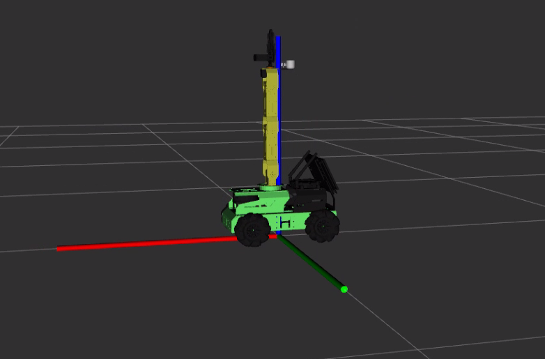
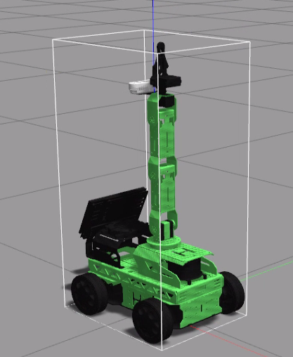
Base Coordinate System

At the base of the robot arm shown in the picture below, consider the bottom servo as the origin. Here, the X-axis is represented by the green axis, the Y-axis by the red axis, and the Z-axis by the blue axis.

Joint Coordinate System

The robotic arm consists of two key components: the rotating joint and the connecting rod. Each joint’s coordinate system is depicted in the model of the robot arm shown below. The origin is represented by the pink cone, with the X-axis in green, the Y-axis in red, and the Z-axis in blue.

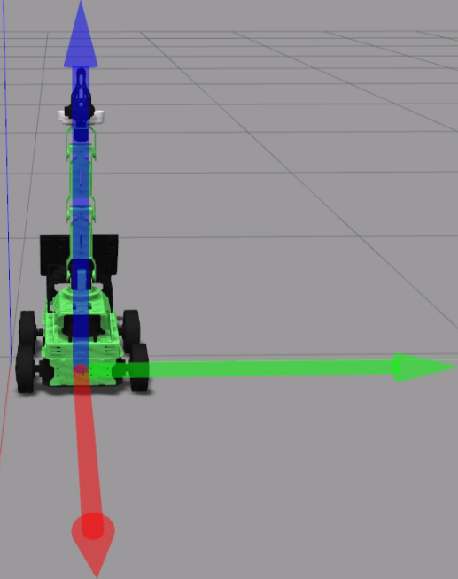
Tool Coordinate System

Tools are typically attached to the end of the robotic arm to fulfill various tasks. The default tool for the robotic arm is the mechanical claw. In the robot arm model shown below, the tool’s coordinate system for the claw has the pink cone position as the origin, with the X-axis represented by green, the Y-axis by red, and the Z-axis by blue.

12.2.7 MoveIt Cartesian Path

MoveIt Cartesian Path Introduction

Cartesian path planning involves planning trajectories in Cartesian space based on the robot’s end effector.

In MoveIt, this method allows you to define the initial and target positions of the robot’s end effector, and it generates a smooth path to move the end effector from the initial position to the target position.

1. Cartesian Coordinate System

The Cartesian coordinate system is a collective term for rectangular and oblique coordinate systems. The two coordinate axes intersecting at the origin form a plane affine coordinate system. If the units of measurement on both axes are equal, this affine coordinate system is called a Cartesian coordinate system. A Cartesian coordinate system in which the two axes are perpendicular is known as a Cartesian rectangular coordinate system; otherwise, it is referred to as a Cartesian oblique coordinate system.

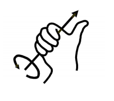
When describing spatial positions, velocities, and accelerations, Cartesian coordinate systems are predominantly employed. When indicating a rotation around a specific axis, the determination of the positive direction follows the right-hand rule, as illustrated in the diagram below:

2. Cartesian Path Planning

Cartesian path planning can be categorized into Cartesian point-to-point path planning and Cartesian continuous path planning based on the nature of the path. In point-to-point planning, the robot’s target point or path is predefined, and the trajectory is obtained by calculating the robot’s joint movements through kinematics. By controlling each axis of the robot in joint space, changes are interpolated independently without considering the movements of other axes. This allows for arbitrary curves between two points.

However, there are cases where the shape of the robot arm’s end trajectory needs to be a straight line or an arc, requiring specific trajectory shapes. In such scenarios, Cartesian path planning with added constraints becomes necessary.

Note

Note: Before starting, ensure there is ample space around the robot. Maintain a safe distance during game to prevent collisions between the robot arm and surroundings, which could cause damage. Also, bend the antenna backward to avoid interference with the robot arm’s movement and potential damage.

This section will introduce Cartesian path constraints to the path planning process, limiting linear motion for both the simulation model and the real manipulator.

3. Cartesian Path Planning Instructions

Set the Motion Group: Start by defining the motion group in MoveIt. A motion group consists of joints that determine the robot’s degrees of freedom and controllable parts. By specifying motion groups, you can constrain degrees of freedom during planning for better control over the robot’s motion.
Set Path Constraints (Optional): If you need to restrict the robot’s motion path, such as maintaining a fixed posture for certain joints, you can apply path constraints. These constraints ensure specific conditions are satisfied during the planning process.
Specify Start and Target Poses: Define the starting and target poses of the robot’s end effector to establish the motion target. These poses are defined using the robot’s coordinate system.
Perform Path Planning: Utilize MoveIt’s path planning interface to generate the Cartesian path for the robot. MoveIt will conduct path planning based on the robot model, constraints, and target poses, producing a smooth path.
Execute Path: Finally, send the generated path to the robot controller for execution. The robot will gradually move to the target pose based on the results of the path planning.

Operation Steps

Note

Note: the input command should be case sensitive, and keywords can be complemented using Tab key.

Start the robot, and access the robot system desktop using remote control software ‘NoMachine’.
Click-on to open the command-line terminal.
Execute the command ‘sudo systemctl stop start_app_node.service’, and hit Enter key to terminate the app auto-start service.
```
sudo systemctl stop start_app_node.service
```
Open a new terminal, and run the command “roslaunch hiwonder_moveit_config demo.launch fake_execution:=false” to launch MoveIt tool.
```
roslaunch hiwonder_moveit_config demo.launch fake_execution:=false
```

The software interface is as below:

①　: RVIZ tool bar;

②　: Movelt debugging area;

③　: Simulation model adjustment area

Locate ‘Planning’ section, and tick ‘Use Cartesian Path’ to enable the Cartesian Path Planning.
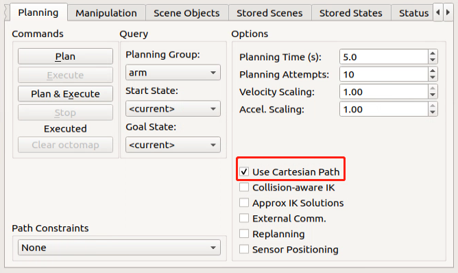
Next, use the mouse to drag the arrow in the ‘Simulation Model Adjustment Area’ to plan the path for the robotic arm. When viewing the robot as the primary perspective, note that:

Green represents the X-axis direction, with the positive direction to the left of the robot.
Red indicates the Y-axis direction, with the positive direction in front of the robot.
Blue signifies the Z-axis direction, with the positive direction above the robot.

After completing the planning, click on ‘Plan & Execute’. The simulation model will then attempt to execute the action by moving the end effector in Cartesian space along a linear path. If the action cannot be achieved due to Cartesian path constraints, a failure message will be displayed.
If you need to terminate this program, use short-cut ‘Ctrl+C’. If the program fails to stop, please retry.

After you’ve finished your gaming experience, you can activate the mobile app service either by using commands or by restarting the robot. If the mobile app service isn’t active, the app’s functions won’t work. (The mobile app service will automatically start if the robot restarts.)

To restart the mobile app service, enter the command: ‘sudo systemctl restart start_app_node.service’. Wait for the robot arm to return to its initial position and for the service startup to complete.

sudo systemctl restart start_app_node.service

12.2.8 MoveIt Collision Detection

MoveIt Collision Detection Description

MoveIt collision detection is a crucial feature that leverages the robot’s motion planning trajectory and environmental object information to identify potential collision scenarios. Its primary aim is to prevent the robot from colliding with nearby objects during its movements.

1. Collision Detection Configuration Introduction

Collision detection in MoveIt2 is configured by CollisionWorld object in planning scene. Collision detection is mainly executed by FCL software pack which is a major CC library for MoveIt2.

2. Collision Object

MoveIt2 welcomes different types of objects to detect collision, including:

Meshes
Basic shape: box, cylinder, cone, sphere and plane.
Octomap—can be directly used in collision detection

3. Allowed Collision Matrix (ACM)

Allowed Collision Matrix (ACM) will encode a binary value to sign whether to detect collision between objects.

If values of these two objects are set as 1, collision detection will not be executed, otherwise collision detection will continue as schedule.

Note

Important Note: Before beginning, ensure there is sufficient space surrounding the robot. Maintain a safe distance from the robot during game to prevent the robot arm from colliding with limbs and causing damage. Additionally, bend the antenna backward to prevent the robot arm from inadvertently moving and colliding with it, thus avoiding damage.

This section will incorporate a collision model to illustrate the impact of collision detection between the simulation model and the actual manipulator.

4. Collision Detection Instructions

Robot Description: Initially, provide the geometric and kinematic details of the robot. Typically, URDF (Unified Robot Description Format) files are utilized to depict the structure and connectivity of the robot. This description encompasses information such as the robot’s joints, links, colliders, and sensors.
Environment Modeling: Model the environment surrounding the robot, including the geometry and positions of obstacles. These obstacles may be either static or dynamic.
Motion Planning: Utilize MoveIt’s motion planner to define the robot’s initial and target postures, thereby generating the robot’s motion trajectory.
Collision Detection: MoveIt conducts collision detection along each posture of the robot within the generated motion trajectory. It employs a robot model and an environment model to compute potential collisions between the robot and obstacles.
Collision Avoidance: Upon detecting a collision, MoveIt adjusts the robot’s posture or path to evade the collision. It iteratively re-plans the robot’s movement path until discovering a collision-free trajectory.

Operation Steps

Note

Note: the input command should be case sensitive, and keywords can be complemented using Tab key.

Start the robot, and access the robot system desktop using remote control software ‘NoMachine’.
Click-on to open the command-line terminal.
Execute the command ‘sudo systemctl stop start_app_node.service’, and hit Enter key to terminate the app auto-start service.
```
sudo systemctl stop start_app_node.service
```
Open a new terminal, and run the command “roslaunch hiwonder_moveit_config demo.launch fake_execution:=false” to launch MoveIt tool.
```
roslaunch hiwonder_moveit_config demo.launch fake_execution:=false
```

The software interface is as below:

RVIZ tool bar;
Movelt debugging area;
Simulation model adjustment area

In the simulation model adjustment area, you will find red, green, and blue arrows. Click and drag these arrows to modify the posture of the robotic arm. When viewing the robot from its perspective, note that green represents the X-axis direction, with the positive direction to the left of the robot; red indicates the Y-axis direction, with the positive direction in front of the robot; and blue signifies the Z-axis direction, with the positive direction above the robot.

After planning the route, the newly determined location will be highlighted in orange, as depicted below:

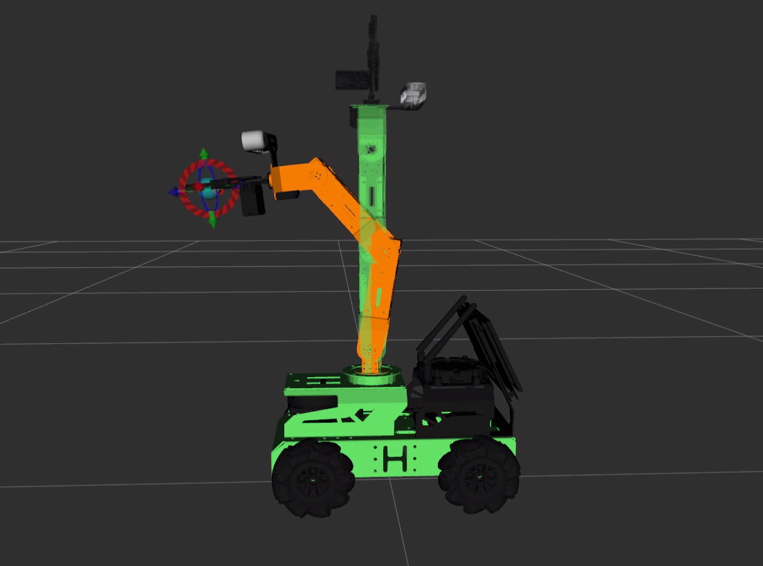
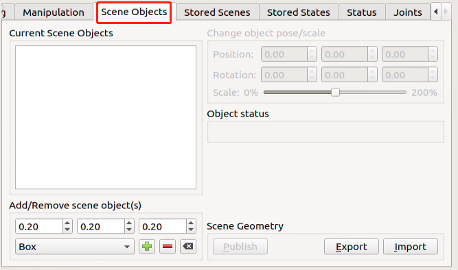
Having finished planning the path of the robot arm, navigate to ‘Scene Objects’ panel to add collision model.
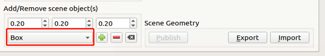
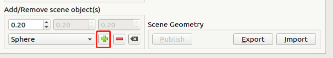
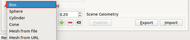
Under the “Box” option, select the collision model of your choice from the dropdown list. As an illustration, we will use the “Sphere” here.
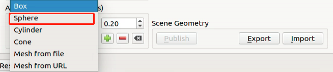
Click-on ‘+’ to add the current model.

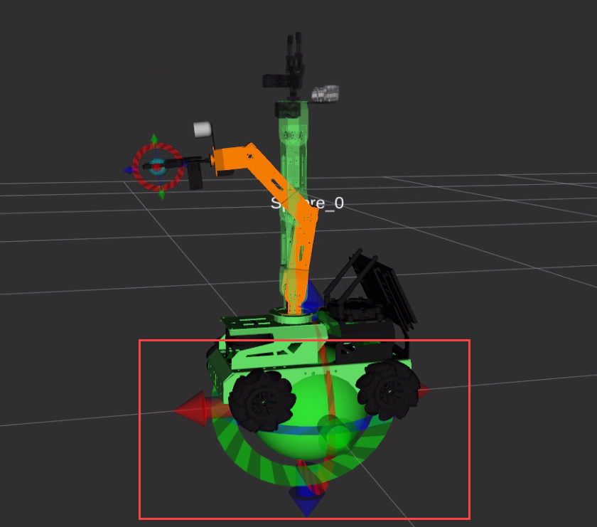
The model will be added to the bottom of the robot by default.
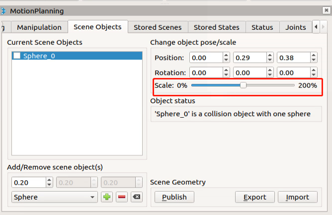
Adjust the size of the collision model by dragging the slider in the illustration below. It is advisable to reduce it to approximately 50% of the original size.
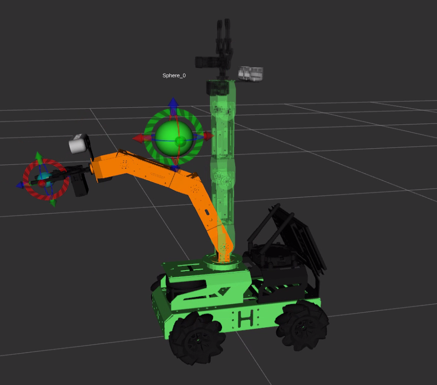
Drag the three-dimensional arrows of the sphere to move the collision model between the starting and target positions for convenient testing of collision detection effects.
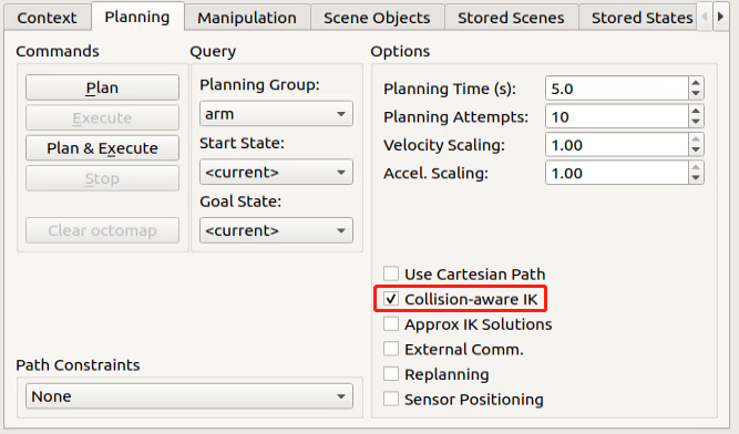
Navigate to the ‘Planning’ section and check ‘Collision-aware IK’ to activate model collision detection.
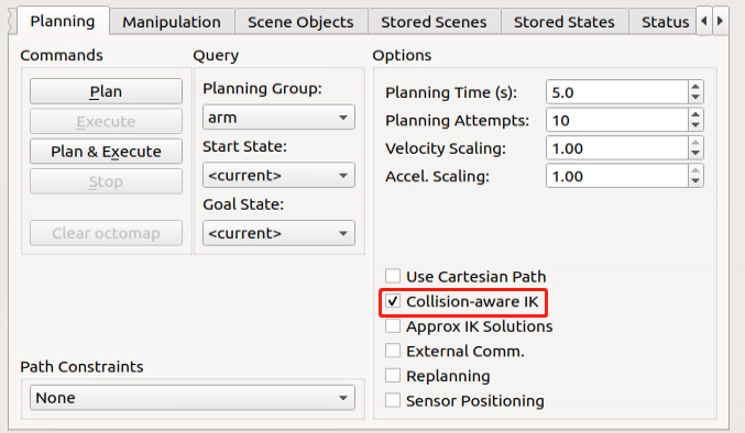
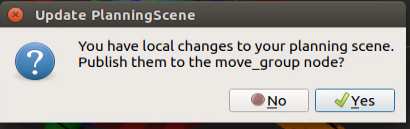
Then, click the ‘Plan&Execute’ button to initiate the movement of the robot arm along the specified path. If you encounter the following prompt, select ‘Yes.’
The robotic arm will plan its movement path, avoiding models along the way to prevent collisions.
If you need to terminate this game, you can use short-cut ‘Ctrl+C’. If the game cannot be shutdown, please retry.

After completing the game experience, you can initiate the mobile app service either through commands or by restarting the robot. It’s essential to note that if the mobile app service is not activated, the relevant app functions will not be available. (The mobile app service will automatically start upon robot restart.)

To restart the mobile app service, enter the command “sudo systemctl restart start_app_node.service”. Wait for the robot arm to return to its initial posture and for the service startup to complete.

sudo systemctl restart start_app_node.service

12.2.9 MoveIt Scenario Design

When using MoveIt for scene design, you have the capability to construct a virtual environment encompassing the robot, obstacles, and target locations. This virtual scene serves multiple purposes, including robot motion planning, collision detection, path optimization, and more.

Scene Design Instructions

Robot Description: Initially, use a URDF file to define the robot’s structure, connections, joint limitations, and other relevant details. This includes specifying the robot’s geometry, kinematic parameters, sensors, etc.

Obstacle Modeling: In scene design, incorporate obstacles to replicate the environment surrounding the robot. These obstacles may be static (e.g., walls, tables, boxes) or dynamic (e.g., moving objects, other robots).

Target Position Setting: Define the target position or posture of the robot within the scene. These targets can represent specific locations the robot needs to reach or tasks it must perform, such as object manipulation or completing specific actions.

Motion Planning: Utilize MoveIt’s motion planner to map out the robot’s trajectory. By inputting the robot’s starting and target positions, MoveIt calculates a smooth path for the robot to navigate from its initial position to the target.

Collision Detection: Throughout the path planning process, MoveIt conducts collision detection checks to ensure the robot avoids collisions with obstacles during movement. If a collision is detected, MoveIt adjusts the path accordingly to find a collision-free trajectory.

Rviz Plug-in Introduction

Rviz is a 3D visualization platform within the ROS system and is one of the plugins of MoveIt. This plugin enables graphical display of external information and can also publish control information to monitoring objects.

Using MoveIt’s Rviz plugin, users can configure a virtual environment (scene), interactively define the initial and target states of the robot, experiment with various motion planning algorithms, and visualize the outcomes.

Note

Note: Prior to starting, ensure adequate space around the robot. Maintain a safe distance from the robot during game to prevent collisions between the robot arm and limbs, avoiding damage. Additionally, bend the antenna backward to prevent the robot arm from colliding with it and causing damage.

Operation Steps

Note

Note: the input command should be case sensitive, and keywords can be complemented using Tab key.

Start the robot, and access the robot system desktop using remote control software ‘NoMachine’.
Click-on to open the command-line terminal.
Execute the command ‘sudo systemctl stop start_app_node.service’, and hit Enter key to terminate the app auto-start service.
```
sudo systemctl stop start_app_node.service
```
Open a new terminal, and run the command “roslaunch hiwonder_moveit_config demo.launch fake_execution:=false” to launch MoveIt tool.
```
roslaunch hiwonder_moveit_config demo.launch fake_execution:=false
```

The software interface is as below:

RVIZ tool bar;
Movelt debugging area;
Simulation model adjustment area
Navigate to the ‘Scene Objects’ section in the debugging area to add a scene object model.
This panel is divided into four sections as follows:
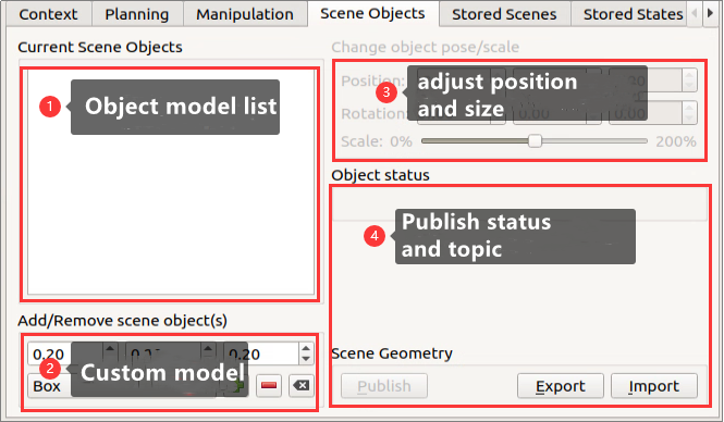
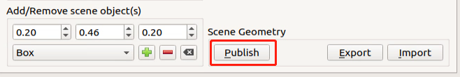
Add basic model, for example Box.
Adjust the size of object model in meter.
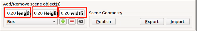
After adjustment, click “+” to add the selected object model to the scene.
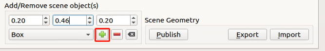
The model list will be updated after you add the model, and the model is generated at the center of the scene i.e. center of robot
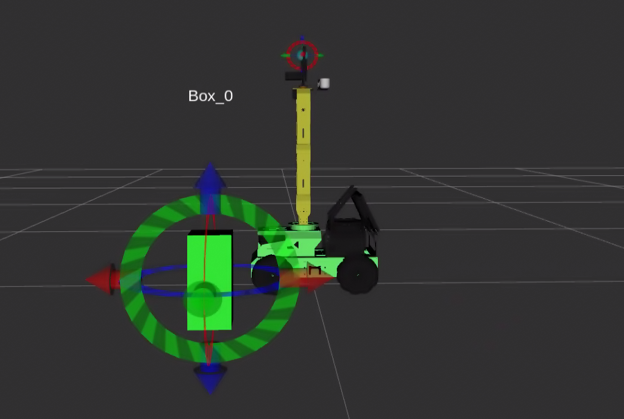
Drag arrows to adjust robotic arm pose.
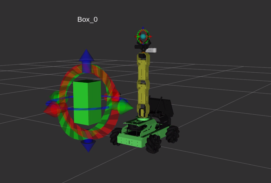
Besides dragging the arrows, adjustments can also be made in the position and size adjustment area.

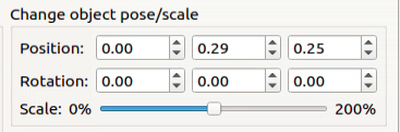
“Position” is to adjust position of object. The boxes from left to right are used to adjust X, Y and Z axis.

“Rotation” is to adjust object angle. The boxes from left to right are used to adjust X, Y and Z axis. “Scale” is to adjust object size.
Click “Publish” after adjustment to publish topic of this model. Movelt will subscribe to this topic automatically.
To protect object model from collision, tick “Collision-aware IK” to start model collision detection.
If you need to terminate this game, you can use short-cut ‘Ctrl+C’. If the game cannot be shutdown, please retry.

After completing the scene design experience, you can initiate the mobile app service either through commands or by restarting the robot. It’s essential to note that if the mobile app service is not activated, the relevant app functions will not be available. (The mobile app service will automatically start upon robot restart.)

To restart the mobile app service, enter the command “sudo systemctl restart start_app_node.service”. Wait for the robot arm to return to its initial posture and for the service startup to complete.

sudo systemctl restart start_app_node.service

12.2.10 MoveIt Trajectory Planning

Motion Planner Introduction

1. Open Motion Planner Library (OMPL)

OMPL is an open robotic motion planner library based on sampling method. Most of algorithms in this library derive from RRT and RPM, for example RRTStar and RRT-Connect.

By virtue of modular design, front-end GUI support and stable update, OMPL is the most mainstream motion planner software. It is default motion planner software of ROS.

A planner that is based on sampling need not take into account dimension of the planning object. That is to say no dimensional explosion will happen. A key reason why it can be used to control robotic arm is that it can effectively tackle path planning problems in high-dimensional space and complex constraints.

For motion planning of N DOF robotic arm, OMPL can plan a trajectory for end effector in robotic arm joint space and create M arrays (trajectory is composed of M control points). Dimension of each array is N (joint sequence of each control point). It can ensure robotic arm will not collide with surrounding obstacles when executing this trajectory.

2. Industrial Motion Planner (Pilz)

Pilz industrial motion planner is a deterministic generator for circular and linear motions. In addition, it also supports integrating multiple motion segments with MoveIt2.

3. Stochastic Trajectory Optimization for Motion Planning（STOMP）

STOMP is a motion planner based on optimization and PI^2 algorithm. This planner can plan smooth trajectories, avoid obstacles and optimize constraints for the robotic arm. Arbitrary terms in the cost function can be optimized since algorithm does not require gradients.

4. Search-based Planning Library (SBPL)

It is a generic set of motion planners using search-based planning to discrete space.

5. Covariant Hamiltonian Optimization for Motion Planning（CHOMP）

CHOMP is an innovative trajectory optimization based on gradient that makes ordinary motion planning simpler and more trainable.

Most high-dimensional motion planners divide the generating process of trajectory into two stages, including planning and optimization. At the stage of optimization, this algorithm employs covariant and functional gradients to design motion planning algorithm that is totally based on trajectory optimization.

Given a infeasible initial trajectory, CHOMP will make quick response to the surroundings so as to make trajectory collision-free, while optimize joint speed and acceleration.

Note

Note: Prior to starting, ensure that there is ample space around the robot. Maintain a safe distance from the robot during gameplay to prevent collisions between the robot arm and limbs, which could cause damage. Additionally, bend the antenna backward to prevent the robot arm from moving and colliding with it, thus avoiding damage.

The program in this section integrates both OMPL and CHOMP planners. By default, the program utilizes the OMPL planner. The following instructions will demonstrate how to activate the CHOMP planner.

Operation Step

Note

Note: the input command should be case sensitive, and keywords can be complemented using Tab key.

Start the robot, and access the robot system desktop using remote control software ‘NoMachine’.
Click-on to open the command-line terminal.
Execute the command ‘sudo systemctl stop start_app_node.service’, and hit Enter key to terminate the app auto-start service.
```
sudo systemctl stop start_app_node.service
```
Launch a new command line terminal and input the following command: “roslaunch hiwonder_moveit_config demo.launch fake_execution:=false pipeline:=chomp” to initialize the MoveIt tool. The parameter “pipeline” designates the trajectory planner, with the default being OMPL. By changing it to “chomp”, CHOMP trajectory planning is enabled.
```
roslaunch hiwonder_moveit_config demo.launch fake_execution:=false pipeline:=chomp
```

The software interface is as below:

RVIZ tool bar;
Movelt debugging area;
Simulation model adjustment area
In the simulation model adjustment area, you’ll find arrows in three colors: red, green, and blue. Click and drag these arrows to modify the posture of the robotic arm. When viewing the robot from its perspective, note that green represents the X-axis direction, with the positive direction to the left of the robot; red indicates the Y-axis direction, with the positive direction in front of the robot; and blue signifies the Z-axis direction, with the positive direction above the robot.
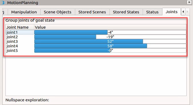
In addition to making overall adjustments using the arrows, you can also individually adjust specific joints. Locate and click the triangle mark on the right-hand side to access the “Joints” panel.
Drag sliders to adjust the joint angle.
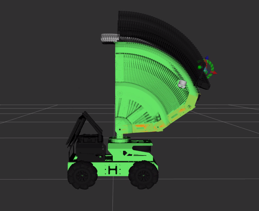
Once the robot arm motion path is successfully planned, the new position will be highlighted in orange. However, if the new position collides with other parts of the robot, it will be marked in red. In such cases, it must be readjusted to a collision-free state; otherwise, the action will not be executed. The figure below illustrates the executable status marked in orange:
Locate the RVIZ toolbar, sequentially click on “Motion Planning” and “Planned Path”, then enable the “Show Trail” option. This will display each frame of the robot arm movement.
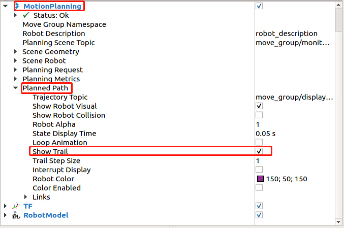
Navigate back to the “Planning” section and select the “Plan” option. The simulation model will illustrate the movement path from the initial position to the newly planned position.
After reviewing the demonstration, deselect “Show Trail”, then proceed to click the “Execute” option. Both the simulation model and robot will simultaneously execute the planned action.
If you need to terminate the program, use short-cut ‘Ctrl+C’. If the program fails to terminate, please retry.

After completing the scene design experience, you can initiate the mobile app service either through commands or by restarting the robot. It’s essential to note that if the mobile app service is not activated, the relevant app functions will not be available. (The mobile app service will automatically start upon robot restart.)

To restart the mobile app service, enter the command “sudo systemctl restart start_app_node.service”. Wait for the robot arm to return to its initial posture and for the service startup to complete.

sudo systemctl restart start_app_node.service

12.3 Gazebo Simulation V1.0

12.3.1 Gazebo Introduction

Simulation software allows for the creation of a realistic virtual physical environment in which robots can be tested and experimented with to observe how they complete tasks. Gazebo is the most widely utilized robot simulation software in ROS (Robot Operating System). Gazebo excels at providing high-fidelity physical simulation conditions and offers an extensive array of sensor models. Moreover, it facilitates seamless interaction between the simulation environment and the robot, thereby enhancing the robot’s performance in intricate settings.

Gazebo supports the use of files in urdf (Unified Robot Description Format) and sdf (Simulation Description Format) formats, which are employed for describing the simulation environment. When working with a hexapod robot, it is common to utilize a urdf model, and the official resources provide a diverse selection of pre-existing models that can be readily employed.

Gazebo GUI Introduction

The interface of simulation software is as below.

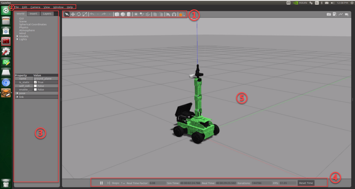
The function of each section on the interface is listed below.

Name	Function
Tool bar (1)	Provide the most commonly used options for interaction with simulator
Menu bar (2)	Configure or modify the parameters of the simulation software and some interactive functions
Action bar (3)	Make any operations on the models and modify the parameters
Timestamp (4)	Set the time of the virtual space
Scene (5)	The main part of the simulator where the simulated model is displayed

To get more info of Gazebo, please visit Gazebo’s official website: http://gazebosim.org/

Gazebo Learning Resources

Gazebo official website: https://gazebosim.org/

Gazebo tutorials: https://gazebosim.org/tutorials

Gazebo GitHub repository: https://github.com/osrf/gazebo

Gazebo Answers Forum: http://answers.gazebosim.org/

12.3.2 Gazebo xacro Model Visualization

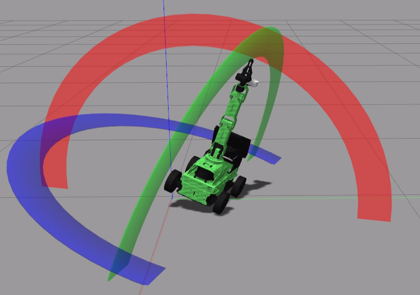
Gazebo can offer an intuitive visualization of robot model and structure.

Start Simulation

Note

Note: the input command should be case sensitive, and keywords can be complemented using Tab key.

Start the robot, and connect it to NoMachine.
Click-on to command-line terminal.
Input command “sudo systemctl stop start_app_node.service” and press Enter to disable app auto-start service.
```
sudo systemctl stop start_app_node.service
```
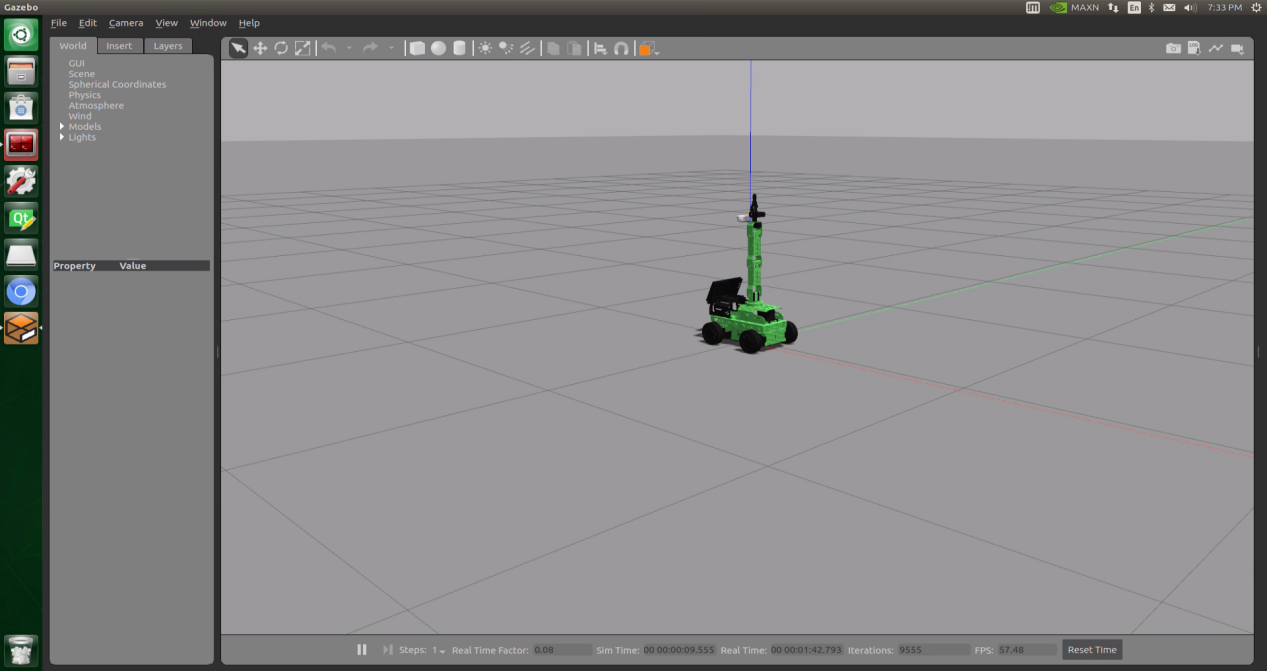
Run the command “roslaunch hiwonder_gazebo worlds.launch” to launch Gazebo.
```
roslaunch hiwonder_gazebo worlds.launch
```
If the below interface appears, it means that Gazebo is opened successfully.

If you encounter difficulties opening the Gazebo simulation model, it could be due to the mobile app service not being closed or other services being enabled. We suggest enabling the mobile app service and closing any other services before executing the command to open the Gazebo simulation model.

Press the shortcut key “Ctrl+C” in the command line terminal window to terminate the currently running program.

Upon completion of the game experience, you can initiate the mobile app service through commands or by restarting the robot. It’s important to note that if the mobile app service is not activated, the relevant app functions will be unavailable. (The mobile app service will automatically start upon robot restart.)

To restart the mobile app service, enter the command “sudo systemctl restart start_app_node.service” and wait for the robot arm to return to its initial posture.

sudo systemctl restart start_app_node.service

The function of each section on the interface is listed below.

Name	Function
Tool bar (1)	Provide the most commonly used options for interaction with simulator
Menu bar (2)	Configure or modify the parameters of the simulation software and some interactive functions
Action bar (3)	Make any operations on the models and modify the parameters
Timestamp (4)	Set the time of the virtual space
Scene (5)	The main part of the simulator where the simulated model is displayed

Shortcut Keys

Left mouse button: In Gazebo simulation, the left mouse button is utilized to drag the map and select targets. You can long-press the left mouse button on the map to move it and click on a model to select it.

Middle mouse button / Shift + left mouse button: By pressing the middle mouse button or holding Shift while clicking the left mouse button, you can rotate the view around the current target point.

Right mouse button / Mouse wheel: Pressing the right mouse button or using the scroll wheel enables you to zoom the map to the position pointed by the mouse cursor.

Tools in the Toolbar (Examples):

Selection Tool : This is Gazebo’s default tool, which allows you to select models in the simulation.

(Note: The introduction of additional tools will be provided separately.)

Move Tool : With the Move tool, you can easily control the movement of a selected model by dragging any of the three axes.
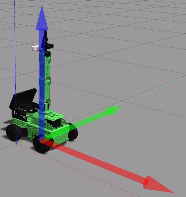
Rotation Tool : The Rotation tool allows you to select a model and then manipulate its rotation by dragging any of the three axes.

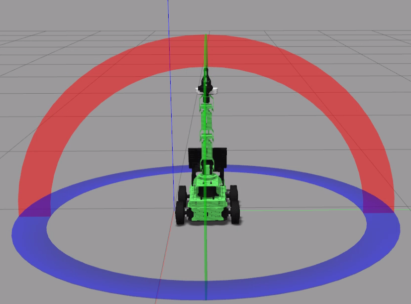
For more detailed information about Gazebo, please visit the official website at http://gazebosim.org/.

12.3.3 Gazebo Hardware Simulation

To comprehend the simulation models of different expansion devices on the robot, it is essential to master corresponding model codes.

Lidar Simulation

Note

Note: the input command should be case sensitive, and keywords can be complemented using Tab key.

Start the robot, and get access to robot system desktop using NoMachine.
Click-on to open command-line terminal.
Execute the command “roscd hiwonder_description/urdf/” and press Enter to navigate to the directory containing programs.
```
roscd hiwonder_description/urdf/
```
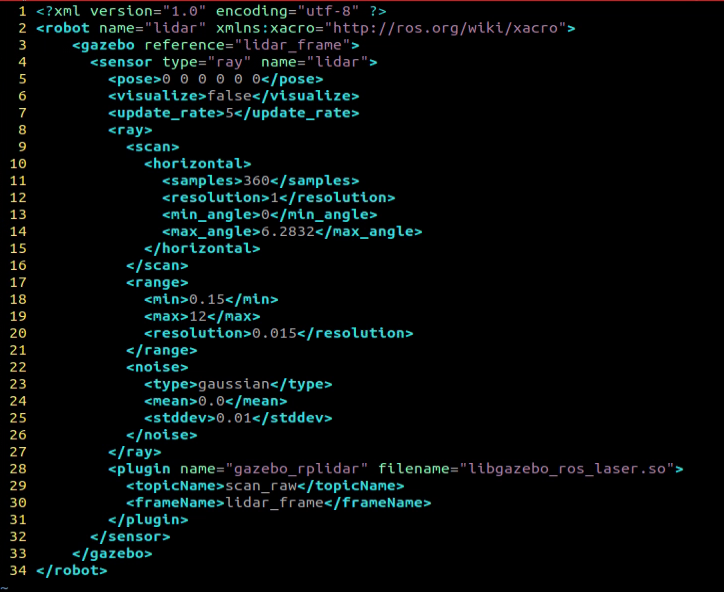
Enter this command “vim lidar.gazebo.xacro” to open Lidar simulation model file.
```
vim lidar.gazebo.xacro
```
This file outlines attributes such as the name, detection range, location, noise reduction settings, and topic message of the lidar simulation model. For further understanding of this file, refer to “12.1 URDF Model Introduction” to learn about the relevant syntax.

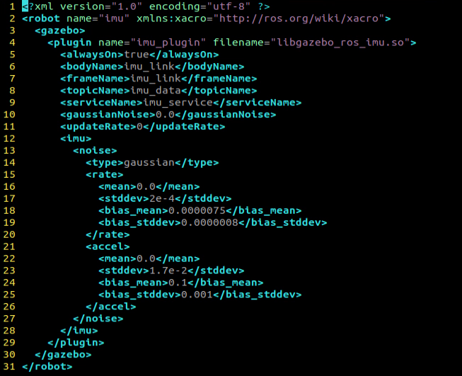
IMU Simulation

Note

Note: the input command should be case sensitive, and keywords can be complemented using Tab key.

Start the robot, and get access to robot system desktop using NoMachine.
Click-on to open command-line terminal.
Execute the command “roscd hiwonder_description/urdf/” and press Enter to navigate to the directory containing programs.
```
roscd hiwonder_description/urdf/
```
Enter this command “vim lidar.gazebo.xacro” to open Lidar simulation model file.
```
vim lidar.gazebo.xacro
```

This file provides details about the lidar simulation model, including its name, detection range, location, noise reduction settings, topic message, and other properties. To gain a better understanding of this document, you can refer to “12.1 URDF Model Introduction” for relevant explanations and syntax rules.

12.3.4 Gazebo Mapping Simulation

Configuration Operation

Note

Note:

Strict case sensitivity is required when entering commands, and the “Tab” key can be used to autocomplete keywords.
Before starting, ensure the handle is prepared and verify that the handle receiver is connected to the robot.

When we aim to create a map within an ideal environment, yet unable to do so in a real-world setting, we can construct the desired scene in Gazebo and simulate mapping.

Start the robot, and get access to robot system desktop using NoMachine.
Click-on to open command-line terminal.
Run the command ‘sudo systemctl stop start_app_node.service’, and hit Enter key to terminate the app auto-start service.
```
sudo systemctl stop start_app_node.service
```

Note

Note: Please ensure each service is fully started before proceeding to start the next one to prevent simulation failure.

Run the command “roslaunch hiwonder_gazebo room_worlds.launch” to enable Gazabo simulation.
```
roslaunch hiwonder_gazebo room_worlds.launch
```
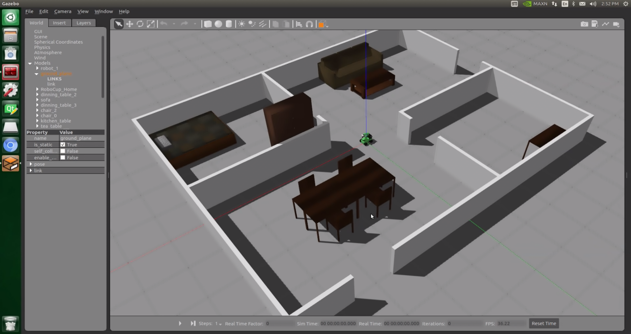
Open a new command-line terminal, and enter the command ‘roslaunch hiwonder_slam slam.launch sim:=true’ to enable the mapping service.
```
roslaunch hiwonder_slam slam.launch sim:=true
```
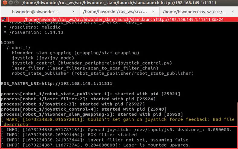
After ensuring the mapping service has fully initialized, return to the Gazebo simulation, click the ‘Start Simulation’ button below, and monitor the information prompts in the mapping service terminal.
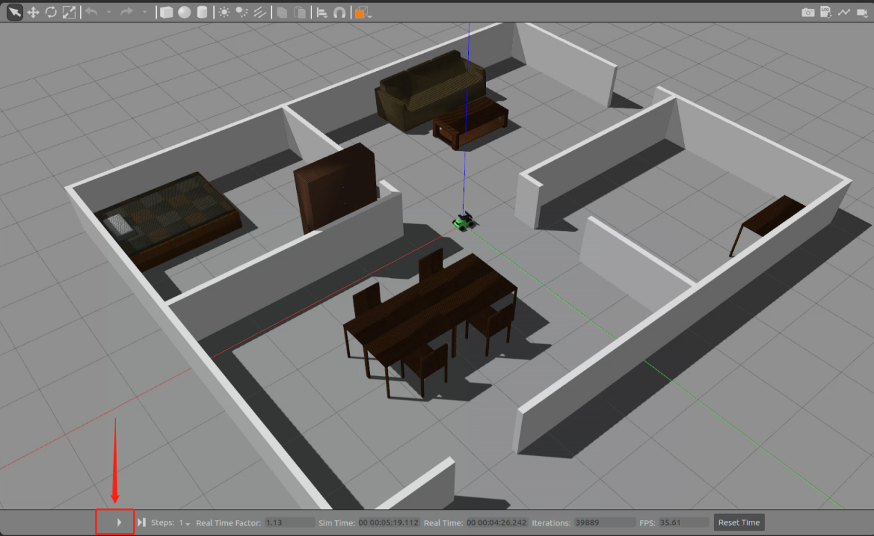
Return to the terminal to observe the following information prompts:

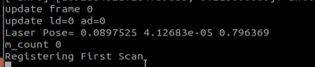
This message provides feedback regarding the current operational status of the mapping service and the progress of data processing.

‘Update frame 0’: Indicates the mapping service is processing data for frame 0. Each update or receipt of robot sensor data increments the frame number.
‘update ld=0 ad=0’: Specifies the number of laser point data (ld) and angle data (ad) detected in the current frame.
‘Laser Pose= 0.0897525 4.12683e-05 0.796369’: Provides the position and orientation information of the lidar, representing its location and direction in the robot coordinate system.
‘m_count 0’: Reflects the number of feature points in the map. As the mapping process progresses, the map is continually updated based on received laser data, leading to an increase in feature points.
‘Registering First Scan’: Indicates the mapping service is registering the initial laser scan data. Typically, the first frame of laser data received during the mapping process is processed and registered to establish an initial map.

Open a new command-line terminal, and run the command ‘roslaunch hiwonder_slam rviz_slam.launch sim:=true’ to launch RVIZ tool.
```
roslaunch hiwonder_slam rviz_slam.launch sim:=true
```
After successful opening, the mapping screen will appear as follows:

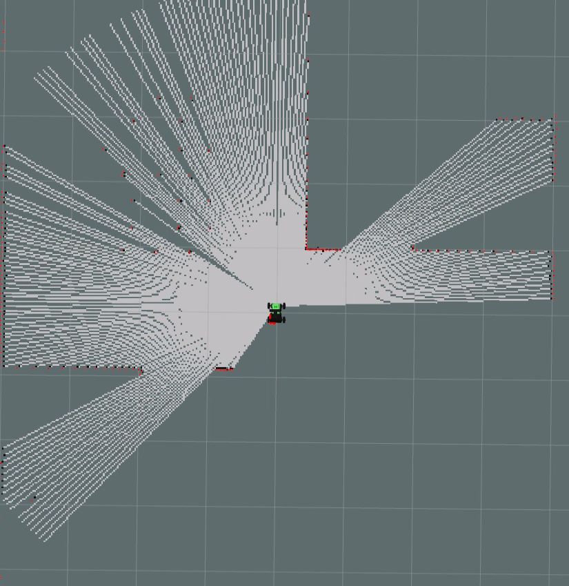
Mapping Instructions

Activate the wireless handle, then use it control the robot to move within the simulation map. The button function of the wireless handle is as listed below:

Button	Function	Description
START	Stop and reset the position	Press briefly
Move left joystick upward	Go forward	Hold and press
Move left joystick downward	Go backward	Hold and press
Move right joystick left	Turn left	Hold and press
Move right joystick right	Turn right	Hold and press

Manipulate the robot to explore within the simulation map, and the mapping result will be displayed simultaneously.
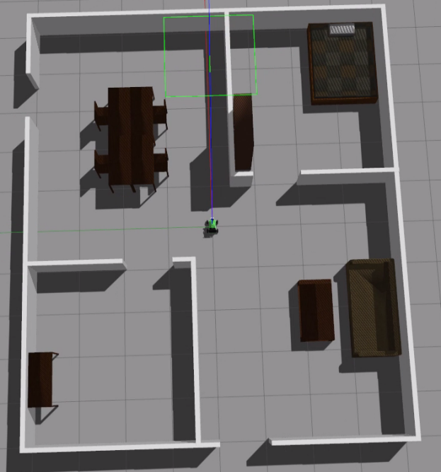
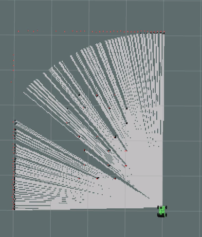
Enter the command ‘roscd hiwonder_slam/maps && rosrun map_server map_saver map:=/robot_1/map -f map_01 ’ to navigate to the directory containing the map.
```
roscd hiwonder_slam/maps && rosrun map_server map_saver map:=/robot_1/map -f map_01
```
The name ‘map_01’ in the command is the identifier for the map, which users can rename as needed. If the following prompt appears, it indicates that the map has been successfully saved.
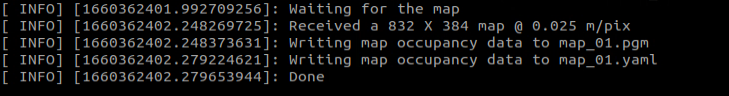
Use the shortcut key “Ctrl+C” in each command line terminal window to terminate the currently running program.

After completing the game experience, you can initiate the mobile app service using commands or by restarting the robot. It’s crucial to ensure that the mobile app service is enabled, as the relevant app functions will not be accessible otherwise. (If the robot is restarted, the mobile app service will start automatically.)

To restart the mobile app service, enter the command “sudo systemctl restart start_app_node.service” and wait for the robot arm to return to its initial posture once the service startup is complete.

sudo systemctl restart start_app_node.service

12.3.5 FAQ

Q: After launching the RVIZ simulation tool, the map is not displayed, only the car model.

A: This issue may arise if multiple services are started simultaneously, leading to congestion in the robot’s processes. We recommend users to press Ctrl+C in the terminal to terminate all processes, then restart the services sequentially, ensuring each service is fully started before proceeding to the next command.

12.3.6 Gazebo Navigation Simulation

When utilizing Gazebo software for mapping, we can navigate within the software scene to simulate the desired effect.

Operation Steps

Note

Note: Strict case sensitivity is required when entering commands, and the “Tab” key can be used to autocomplete keywords.

Start the robot, and access the robot system using the remote control software NoMachine.
Click-on to open the command-line terminal.
Execute the command ‘sudo systemctl stop start_app_node.service’, and hit Enter key to terminate the app auto-start service.
```
sudo systemctl stop start_app_node.service
```

Note

Note: Please ensure each service is fully started before proceeding to start the next one to prevent simulation failure.

Type the command ‘roslaunch hiwonder_gazebo room_worlds.launch’ to access the simulation map.
```
roslaunch hiwonder_gazebo room_worlds.launch
```
Open a command-line terminal, and run the command ‘roslaunch hiwonder_navigation navigation.launch sim:=true map:=map_01’ to load the required map and enable navigation.
```
roslaunch hiwonder_navigation navigation.launch sim:=true map:=map_01
```

The parameter ‘map_01’ at the end of the command represents the name of the map, which users can adjust according to their requirements. The storage path of the map is “/home/ros_ws/src/hiwodner_slam/maps”.

Open a new command-line terminal, and execute the command ‘roslaunch hiwonder_navigation rviz_navigation.launch sim:=true’ to launch the RVIZ tool.
```
roslaunch hiwonder_navigation rviz_navigation.launch sim:=true
```
Click-on to activate the simulation.

The navigation interface is as below after the navigation service is enabled successfully.

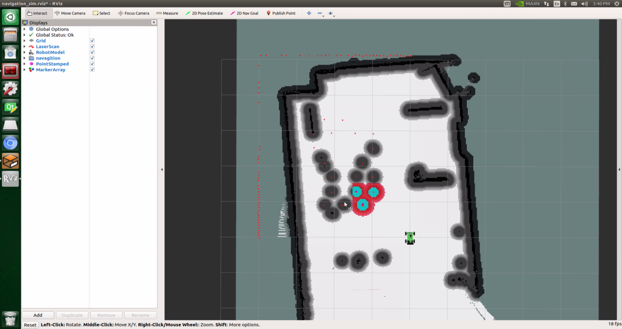
Enable Navigation

In the software menu bar, there are three tools: 2D Pose Estimate, 2D Nav Goal, and Publish Point.

“2D Pose Estimate” is used to define the initial position of the robot.

“2D Nav Goal” is utilized to designate a single target point for the robot.

“Publish Point” is employed to specify multiple target points for the robot.

Select the ‘2D Nav Goal’ tool from the software menu bar, then click on the map interface to designate a point as the target location. Alternatively, you can press and drag the mouse to specify the direction for the robot after reaching the target point. Once the selection is finalized, the robot will automatically generate a route and navigate to the designated target point.

After determining the target point, the map will showcase the planned path of the robot, and the simulation model of the robot will move to the designated position accordingly.

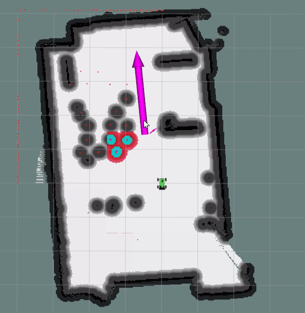
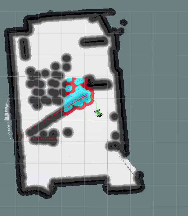
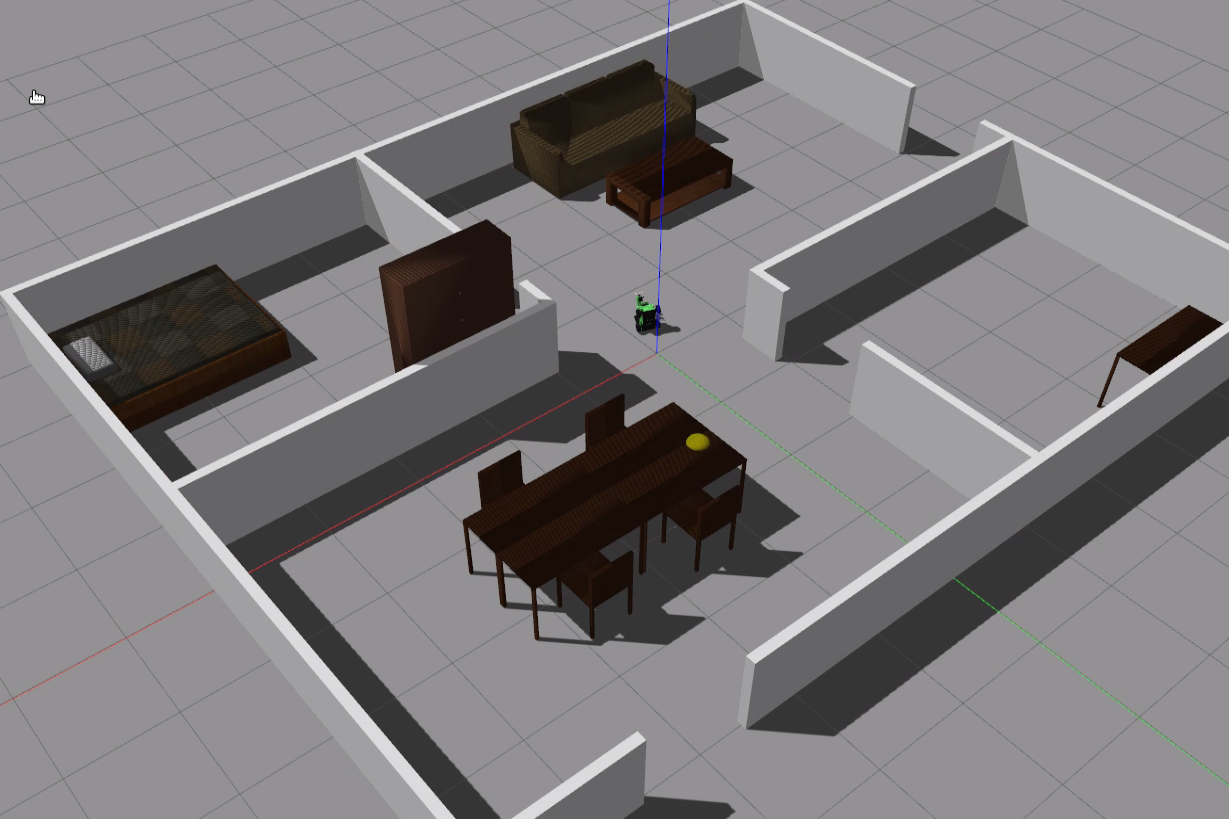
To utilize the multi-point navigation function, open a new terminal and execute the command “roslaunch hiwonder_navigation publish_point.launch”. Wait until the command is successfully executed before proceeding with the multi-point navigation function.
Click and left-click on a specific point on the map interface to set it as a target point. Subsequent target points can be set in a similar manner. After setting the target points, the robot will automatically generate a travel route based on the sequence of the designated target points, navigating to each point sequentially.

Note

Note: It’s necessary to click “Publish Point” once before setting each target point.

To conclude the navigation function, return to the terminal interface and press “Ctrl+C” in each terminal to terminate the processes.
Upon completion of the gameplay experience, users can initiate the mobile app service via instructions or restart the robot. It’s essential to ensure that the mobile app service is activated, as the relevant app functions will not be available otherwise. (If the robot is restarted, the mobile app service will automatically start.)
Enter the command “sudo systemctl restart start_app_node.service” to restart the mobile app service, and wait for the robot arm to return to its initial posture once the service startup is complete.
```
sudo systemctl restart start_app_node.service
```